7.3 CompTox Dashboard Data through APIs
This training module was developed by Paul Kruse and Caroline Ring, with contributions from Julia E. Rager. It was updated and edited November 2025.
All input files (script, data, and figures) can be downloaded from the UNC-SRP TAME2 GitHub website.
Disclaimer: The views expressed in this document are those of the authors and do not necessarily reflect the views or policies of the U.S. EPA.
Introduction to Training Module
Environmental health research related to chemical exposures often requires accessing and wrangling chemical-specific data. The CompTox Chemicals Dashboard (CCD), developed by the United States Environmental Protection Agency, is a publicly-accessible database that integrates chemical data from multiple domains. Chemical data available on the CCD include physicochemical, environmental fate and transport, exposure, toxicokinetics, functional use, in vivo toxicity, in vitro bioassay, and mass spectra data. The CCD was first described in Williams et al. (2017), and has been continuously expanded since. The CCD is heavily used by researchers who do cheminformatics work of various kinds – computational toxicology, computational exposure science, analytical chemistry, chemical safety assessment, etc. The CCD is used by cheminformaticians not only at EPA, but across governmental agencies both within the U.S. and worldwide; in private industry; in non-governmental organizations; in academia; and others. It has become an indispensable tool for many researchers.
This training module provides an overview of the physico-chemical, hazard, and bioactivity data available through the CCD; different ways to access these data; and some examples of how these data may be used. We will first introduce the CCD and how to access it. Then we will focus on an automated, programmatic method for retrieving data from the CCD using the ctxR R package. Through some basic data visualization and analysis using the R programming language, we will explore some data retrieved from the CCD, and gain insights both in how to wrangle the data and combine different methods of accessing the data to build automated pipelines for use in more complex settings.
Note, as the ctxR package accesses data that is periodically updated, some code chunks will produce numbers that may change slightly with data updates. Keep this in mind when running these code chunks in the future.
Training Module’s Environmental Health Questions
This training module was specifically developed to answer the following questions:
After automatically pulling the fourth Drinking Water Contaminant Candidate List from the CompTox Chemicals Dashboard, list the properties and property types present in the data. What are the mean values for a specific property when grouped by property type and when ungrouped?
The physico-chemical property data are reported with both experimental and predicted values present for many chemicals. Are there differences between the mean predicted and experimental results for a variety of physico-chemical properties?
After pulling the genotoxicity data for the different environmental contaminant data sets, list the assays associated with the chemicals in each data set. How many unique assays are there in each data set? What are the different assay categories and how many unique assays for each assay category are there?
The genotoxicity data contains information on which assays have been conducted for different chemicals and the results of those assays. How many chemicals in each data set have a ‘positive’, ‘negative’, and ‘equivocal’ value for the assay result?
Based on the genotoxicity data reported for the chemical with DTXSID identifier DTXSID0020153, how many assays resulted in a positive/equivocal/negative value? Which of the assays were positive and how many of each were there for the most reported assays?
After pulling the hazard data for the different data sets, list the different exposure routes for which there is data. What are the unique risk assessment classes for hazard values for the oral route and for the inhalation exposure route? For each such exposure route, which risk assessment class is most represented by the data sets?
There are several types of toxicity values for each exposure route. List the unique toxicity values for the oral and inhalation routes. What are the unique types of toxicity values for the oral route and for the inhalation route? How many of these are common to both the oral and inhalation routes for each data set?
When examining different toxicity values, the data may be reported in multiple units. To assess the relative hazard from this data, it is important to take into account the different units and adjust accordingly. List the units reported for the cancer slope factor, reference dose, and reference concentration values associated with the oral and inhalation exposure routes for human hazard. Which chemicals in each data set have the highest cancer slope factor, lowest reference dose, and lowest reference concentration values?
Script Preparations
Loading R Packages
# Used to interface with CompTox Chemicals Dashboard
library(ctxR)
#> ℹ CCTE's Terms of Service: <https://www.epa.gov/comptox-tools/computational-toxicology-and-exposure-apis>
#> ℹ Please cite ctxR if you use it! Use `citation('ctxR')` for details.
#> No config file or environment variable found: API access unlikely.

# Used to visualize data in a variety of plot designs
library(ggplot2)
Introduction to CompTox Chemicals Dashboard
Accessing chemical data and wrangling it is a vital step in many types of workflows related to chemical, biological, and environmental modeling. While there are many resources available from which one can pull data, the CompTox Chemicals Dashboard built and maintained by the United States Environmental Protection Agency is particularly well-designed and suitable for these purposes. Originally introduced in The CompTox Chemistry Dashboard: a community data resource for environmental chemistry, the CCD contains information on over 1.2 million chemicals as of December 2023.
The CCD includes chemical information from many different domains, including physicochemical, environmental fate and transport, exposure, usage, in vivo toxicity, and in vitro bioassay data (Williams et al., 2017).
The CCD can be searched either one chemical at a time, or using a batch search.
Searching One Chemical at a Time (Single-substance Search)
In single-substance search, the user types a full or partial chemical identifier (name, CASRN, InChiKey, or DSSTox ID) into a search box on the CCD homepage. Autocomplete provides a list of possible matches; the user selects one by clicking on it, and is then taken to the CCD page for that substance. Here is an example of the CCD page for the chemical Bisphenol A:
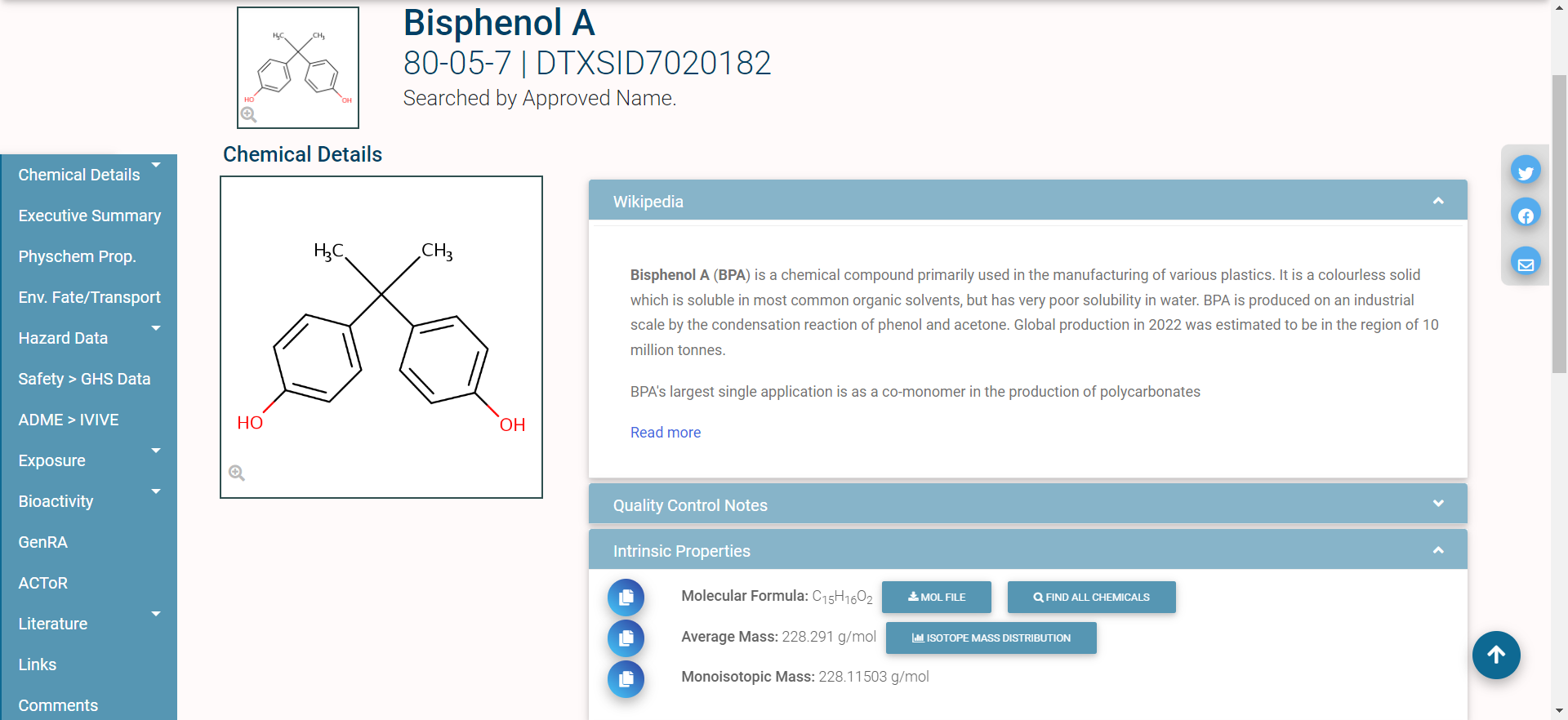
The different domains of data available for this chemical are shown by the tabs on the left side of the page: for example, “Physchem Prop.” (physico-chemical properties), “Env. Fate/Transport” (environmental fate and transport data), and “Hazard Data” (in vivo hazard and toxicity data), among others.
Batch Search
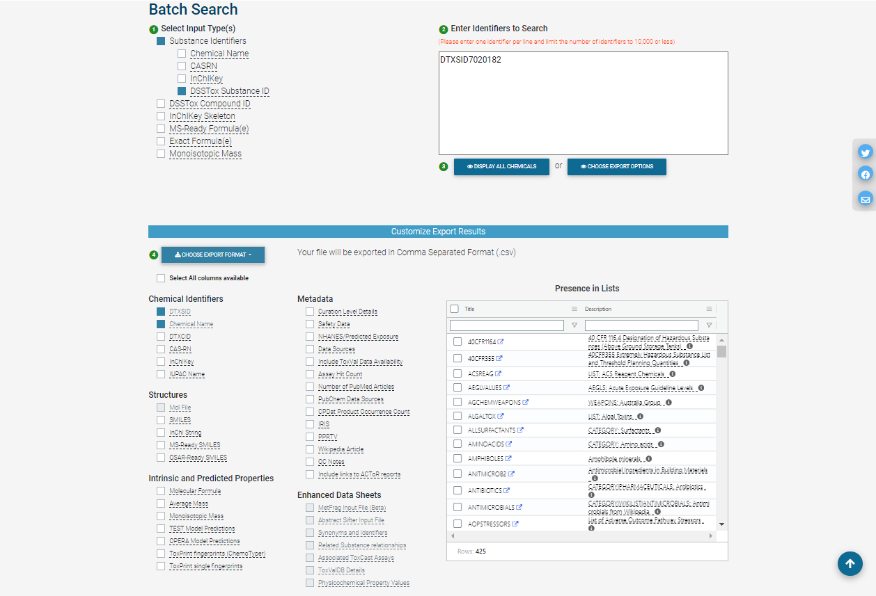
In batch search, the user enters a list of search inputs, separated by newlines, into a batch-search box on https://comptox.epa.gov/dashboard/batch-search . The user selects the type(s) of inputs by selecting one or more checkboxes – these may include chemical identifiers, monoisotopic masses, or molecular formulas. Then, the user selects “Display All Chemicals” to display the list of substances matching the batch-search inputs, or “Choose Export Options” to choose options for exporting the batch-search results as a spreadsheet. The exported spreadsheet may include data from most of the domains available on an individual substance’s CCD page.
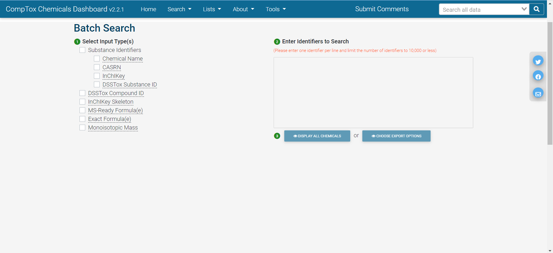
The user can download the selected information in various formats, such as Excel (.xlsx), comma-separated values (.csv), or different types of chemical table files (.e.g, MOL).
The web interface for batch search only allows input of 10,000 identifiers at a time. If a user needs to retrieve information for more than 10,000 chemicals, they will need to separate their identifiers into multiple batches and search each one separately.
Challenges of Web-based Dashboard Search
Practicing researchers typically end up with a Dashboard workflow that looks something like this:
- Start with a dataset that includes your chemical identifiers of interest. These may include chemical names, Chemical Abstract Service Registry Numbers (CASRNs), Distributed Searchable Structure-Toxicity Database (DSSTox) identifiers, or InChIKeys.
- Export the chemical identifiers to a spreadsheet. Often, this is done by importing the data into an environment such as R or Python, in order to do some data wrangling (e.g., to select only the unique substance identfiers; to clean up improperly-formatted CASRNs; etc.). Then, the identifiers are saved in a spreadsheet (an Excel, .csv, or .txt file), one chemical identifier per row.
- Copy and paste the chemical identifiers from the spreadsheet into the CCD Batch Search box. If there are more than 10,000 total chemical identifiers, divide them into batches of 10,000 or less, and search each batch separately.
- Choose your desired export options on the CCD Batch Search page.
- Download the exported spreadsheet of CCD data. By default, the downloaded spreadsheet will be given a file name that includes the timestamp of the download.
- Repeat steps 3-5 for each batch of 10,000 identifiers produced in step 2.
- Import the downloaded spreadsheet(s) of CCD data into the analysis tool you are using (e.g. R or Python).
- Merge the table(s) of downloaded CCD data with your original dataset of interest.
- Proceed with research-related data analysis using the chemical data downloaded from the CCD (e.g., statistical modeling, visualization, etc.)
Because each of these workflow steps requires manual interaction with the search and download process, the risk of human error inevitably creeps in. Here are a few real-world possibilities (the authors can neither confirm nor deny that they have personally committed any of these errors):
- Researchers could copy/paste the wrong identifiers into the CCD batch search, especially if they have more than 10,000 identifiers and have to divide them into batches.
- Chemical identifiers could be corrupted during the process of exporting to a spreadsheet. For example, if a researcher opens and resaves a CSV file using Microsoft Excel, any information that appears to be in date-like format will be automatically converted to a date (unless the researcher has the most recently-updated version of Excel and has selected the option in Settings that will stop Excel from auto-detecting dates). This behavior has long been identified as a problem in genomics, where gene names can appear date-like to Excel (Abeysooriya et al. 2021). It also affects cheminformatics, where chemical identifiers can appear date-like to Excel. For example, the valid CASRN “1990-07-4” would automatically be converted to “07/04/1990” (if Excel is set to use MM/DD/YYYY date formats). CCD batch search cannot recognize “07/04/1990” as a valid chemical identifier and will be unable to return any chemical data.
- Researchers could accidentally rename a downloaded CCD data file to overwrite a previous download (for example, when searching multiple batches of identifiers).
- Researchers could mistakenly import the wrong CCD download file back into their analysis environment (for example, when searching multiple batches of identifiers).
Moreover, the manual stages of this kind of workflow are also non-transparent and not easily reproducible.
CCTE’s CTX Application Programming Interfaces (APIs) for Automated Batch Search of the CCD
Recently, the Center for Computational Toxicology and Exposure (CCTE) developed a set of Application Programming Interfaces (APIs) that allows programmatic access to the CCD, bypassing the manual steps of the web-based batch search workflow. The Computational Toxicology and Exposure (CTX) APIs effectively automate the process of accessing and downloading data from the web pages that make up the CCD.
The CTX APIs are publicly available at no cost to the user. However, in order to use the CTX APIs, you must have an API key. The API key uniquely identifies you to the CTX servers and verifies that you have permission to access the database. Getting an API key is free, but requires contacting the API support team at ccte_api@epa.gov.
For more information on the data accessible through the CTX APIs and related tools, please visit the US EPA page on Computational Toxicology and Exposure Online Resources. The CTX APIs are one of many resources developed within this research realm and make available many of the data resources beyond the CCD.
The APIs are organized into four sets of “endpoints” (chemical data domains): Chemical, Hazard, Bioactivity, and Exposure. Pictured below is what the Chemical section looks like and can be found at CTX API Chemical Endpoints.
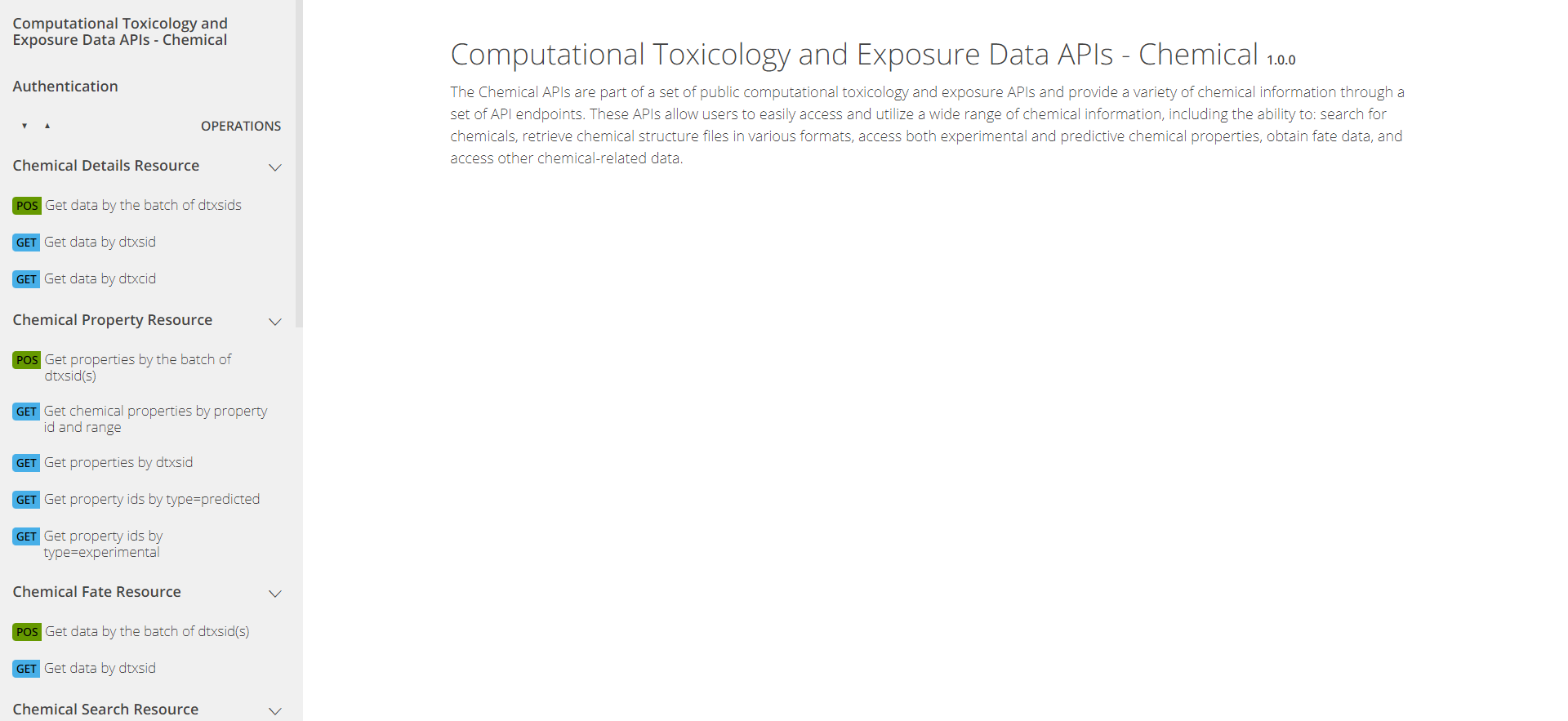
The APIs can be explored through the pictured web interface at https://api-ccte.epa.gov/docs/chemical.html .
CTX API Authentication
Authentication is the first tab on the left. Authentication is required to use the APIs. To authenticate yourself in the API web interface, input your unique API key.
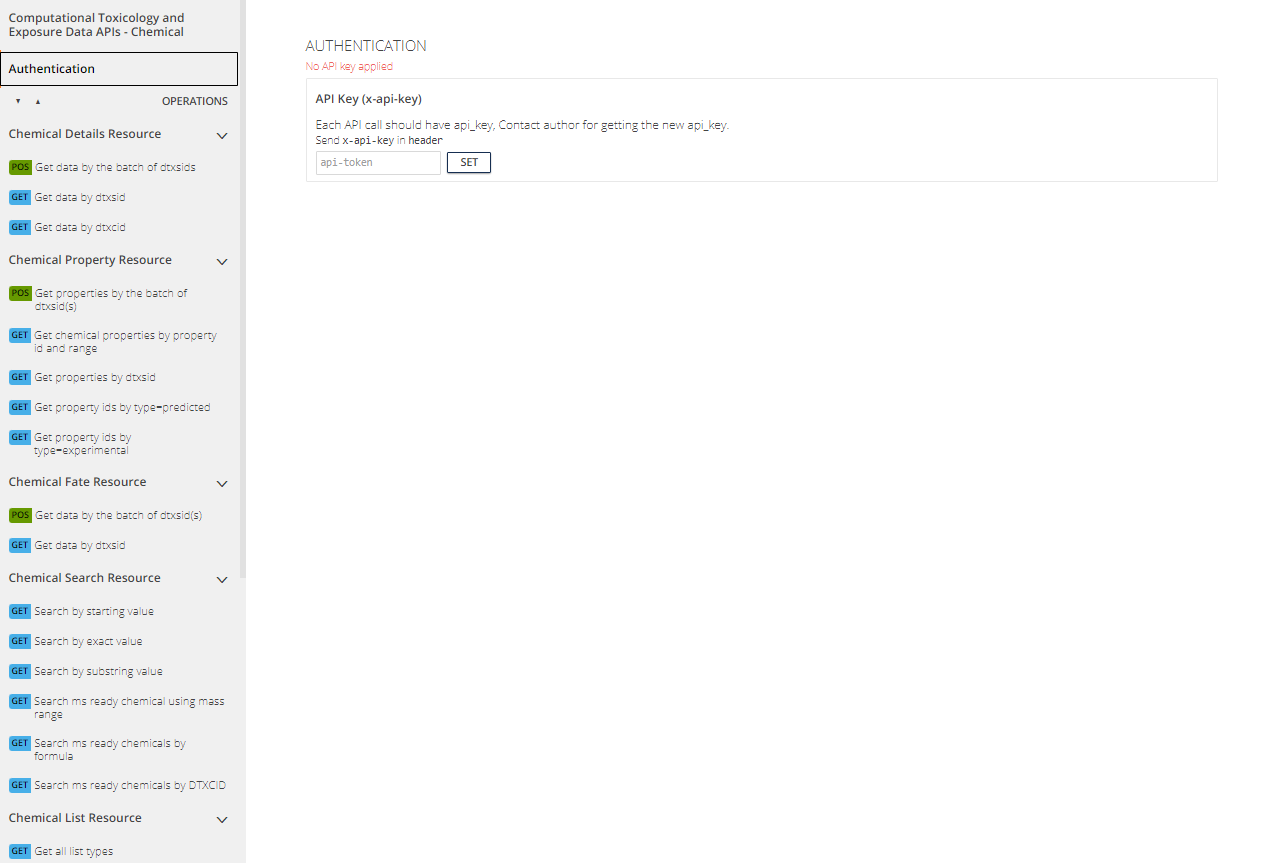
CTX API Endpoints
On the left of the API web interface, there are several different tabs, one for each endpoint in the Chemical domain. The endpoints are organized by the type of information provided. For instance, the Chemical Details Resource endpoint provides basic chemical information; the Chemical Property Resource endpoint provides more comprehensive physico-chemical property information; the Chemical Fate Resource endpoint provides chemical fate and transport information; and so on.
Constructing CTX API Requests
As mentioned above, APIs effectively automate the process of accessing and downloading data from the web pages that make up the CCD. APIs do this by automatically constructing requests using the Hypertext Transfer Protocol (HTTP) that enables communication between clients (e.g. your computer) and servers (e.g. the CCD).
In the CTX API web interface, the colored boxes next to each endpoint indicate the type of the associated HTTP method: either a GET request (“GET”, blue) or a a POST request (“POS”, green). GET is used to request data from a specific web resource (e.g. a specific URL); POST is used to send data to a server to create or update a web resource. For the CTX APIs, POST requests are used to perform multiple (batch) searches in a single API call; GET requests are used for non-batch searches. You do not need to understand the details of POST and GET requests in order to use the API.
Click on the second item under Chemical Details Resource, the tab labeled Get data by dtxsid. The following page will appear.
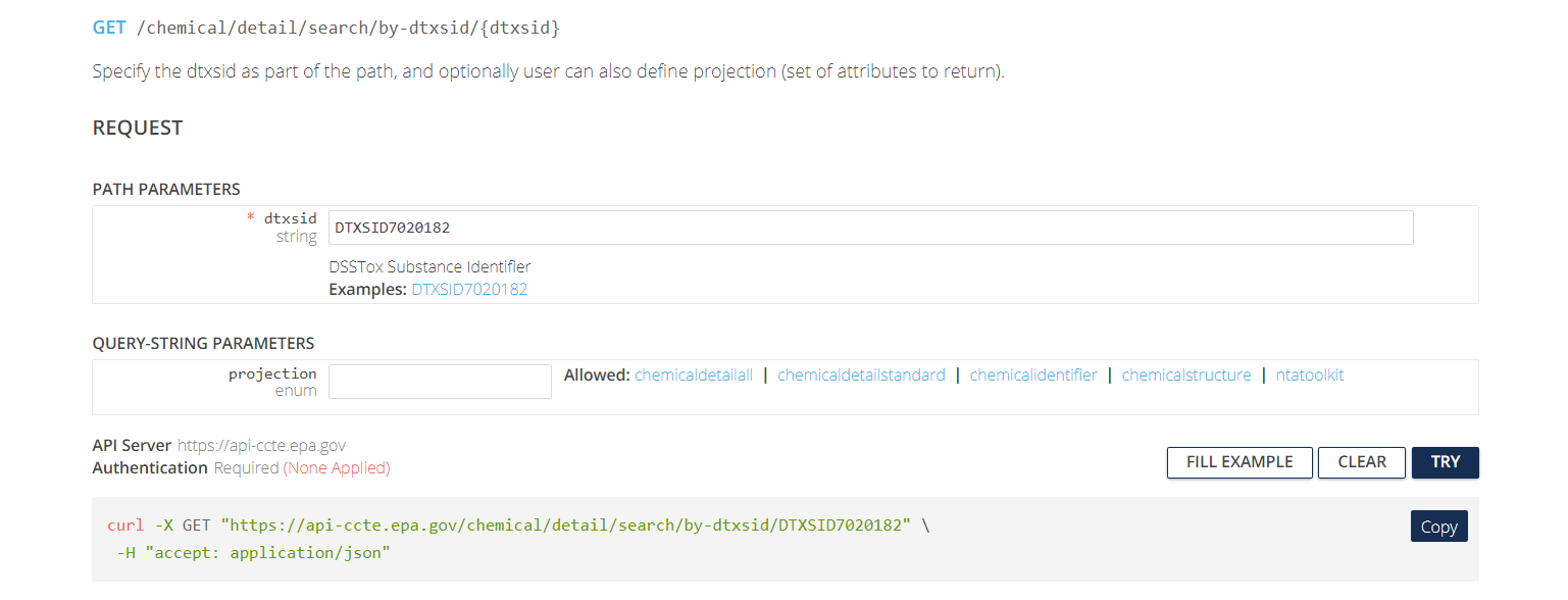
This page has two subheadings: “Path Parameters” and “Query-String Parameters”. “Path Parameters” contains user-specified parameters that are required in order to tell the API what URL (web address) to access. In this case, the required parameter is a string for the DTXSID identifying the chemical to be searched.
“Query-String Parameters” contain user-specific parameters (usually optional) that tell the API what specific type(s) of information to download from the specified URL. In this case, the optional parameter is a projection parameter, a string that can take one of five values (chemicaldetailall, chemicaldetailstandard, chemicalidentifier, chemicalstructure, ntatoolkit). Depending on the value of this string, the API can return different sets of information about the chemical. If the projection parameter is left blank, then a default set of chemical information is returned.
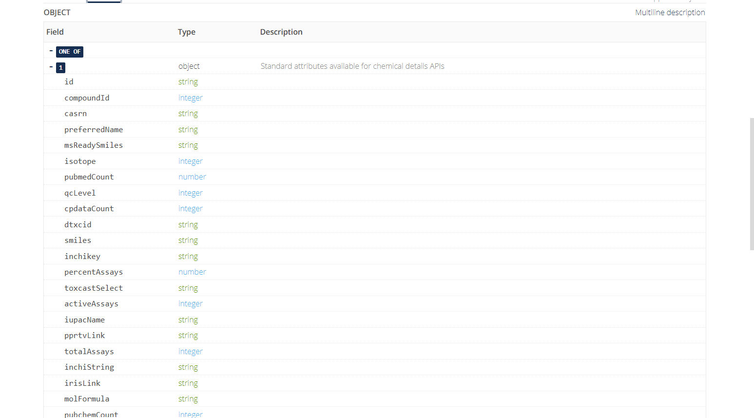
The default return format is displayed below and includes a variety of fields with data types represented.
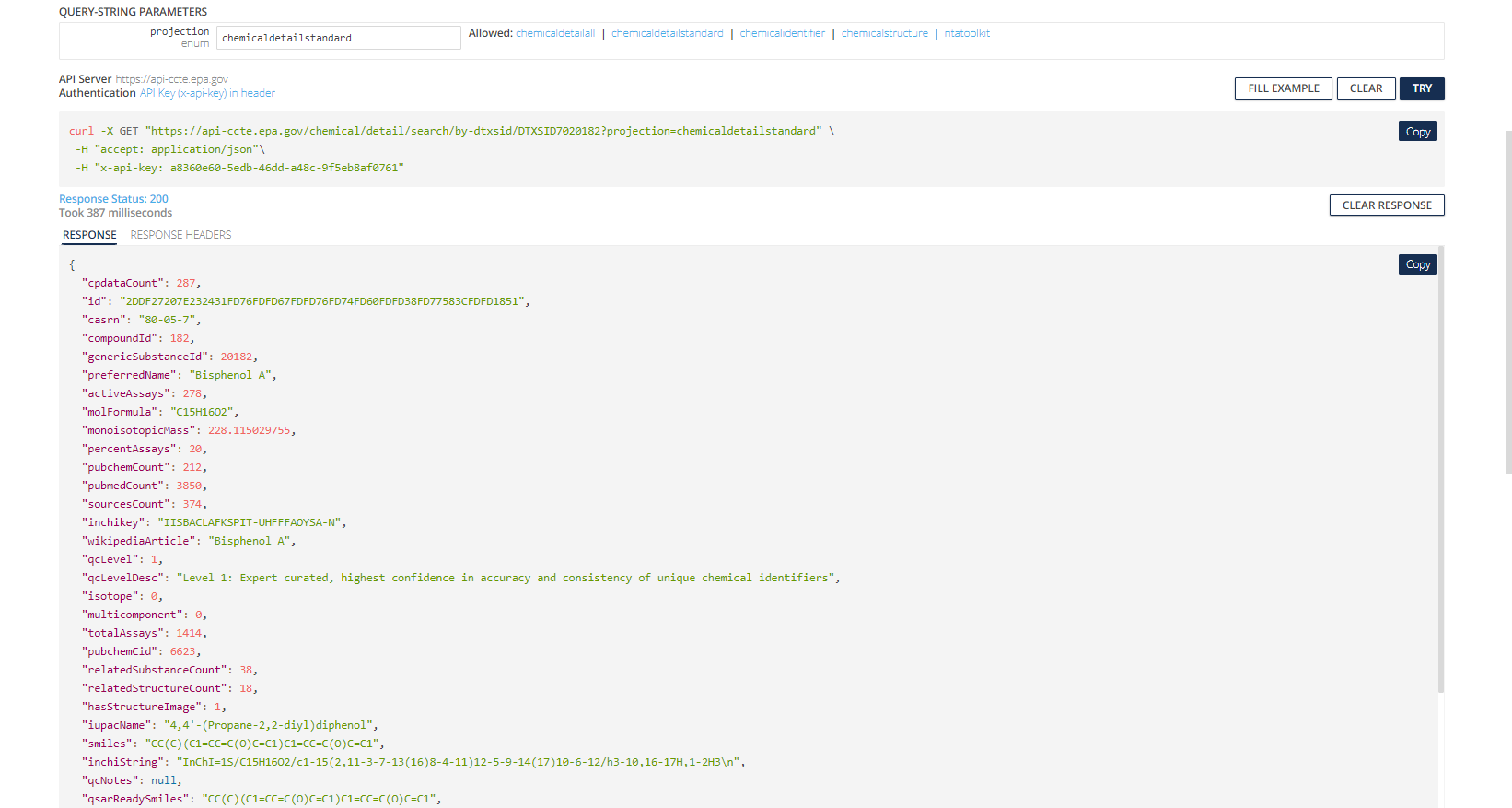
We show what reRturned data from searching Bisphenol A looks like using this endpoint with the chemicaldetailstandard value for projection selected.
Formatting an http request is not necessarily intuitive nor worth the time for someone not already familiar with the process, so these endpoints may provide a resource that for many would require a significant investment in time and energy to learn how to use. However, there is a solution to this in the form of the R package ctxR.
ctxR was developed to streamline the process of accessing the information available through the CTX APIs without requiring prior knowledge of how to use APIs. The ctxR package is available in stable form on CRAN and a development version may be found at the USEPA ctxR GitHub repository. As an example, we demonstrate the ease with which one may retrieve the information given by this endpoint for Bisphenol A using the ctxR approach and contrast it with the approach using the CCD website or CTX Chemical API Endpoint website.
Setting, using, and storing the API key
We store the API key required to access the APIs. To do this for the current session, run the first command. If you want to store your key across multiple sessions, run the second command.
# This stores the key in the current session
register_ctx_api_key(key = '<YOUR API KEY>')

# This stores the key across multiple sessions and only needs to be run once.
# If the key changes, rerun this with the new key.
register_ctx_api_key(key = '<YOUR API KEY>', write = TRUE)
To check that your key has successfully been stored for the session, run the following command.
Retrieving chemical details
Now, we demonstrate how to retrieve the information for BPA given by the Chemical Detail Resource endpoint under the chemicaldetailstandard value for projection. Note, this projection value is the default value for the function get_chemical_details().
BPA_chemical_detail <- get_chemical_details(DTXSID = 'DTXSID7020182')
dim(BPA_chemical_detail)
#> [1]  1 37
class(BPA_chemical_detail)
#> [1] "data.table" "data.frame"
names(BPA_chemical_detail)
#>  [1] "id"                    "cpdataCount"           "inchikey"
#>  [4] "wikipediaArticle"      "monoisotopicMass"      "percentAssays"
#>  [7] "pubchemCount"          "pubmedCount"           "sourcesCount"
#> [10] "qcLevel"               "qcLevelDesc"           "isotope"
#> [13] "multicomponent"        "totalAssays"           "pubchemCid"
#> [16] "relatedSubstanceCount" "relatedStructureCount" "casrn"
#> [19] "compoundId"            "genericSubstanceId"    "preferredName"
#> [22] "activeAssays"          "molFormula"            "hasStructureImage"
#> [25] "iupacName"             "smiles"                "inchiString"
#> [28] "qcNotes"               "qsarReadySmiles"       "msReadySmiles"
#> [31] "irisLink"              "pprtvLink"             "descriptorStringTsv"
#> [34] "isMarkush"             "dtxsid"                "dtxcid"
#> [37] "toxcastSelect"
Comparing Physico-chemical Properties between Two Important Environmental Contaminant Lists
We study two different data sets contained in the CCD and observe how they relate and how they differ. The two data sets that we will explore are a water contaminant priority list and an air toxics list.
The fourth Drinking Water Contaminant Candidate List (CCL4) is a set of chemicals that “…are not subject to any proposed or promulgated national primary drinking water regulations, but are known or anticipated to occur in public water systems….” Moreover, this list “…was announced on November 17, 2016. The CCL 4 includes 97 chemicals or chemical groups and 12 microbial contaminants….” The National-Scale Air Toxics Assessments (NATA) is “… EPA’s ongoing comprehensive evaluation of air toxics in the United States… a state-of-the-science screening tool for State/Local/Tribal agencies to prioritize pollutants, emission sources and locations of interest for further study in order to gain a better understanding of risks… use general information about sources to develop estimates of risks which are more likely to overestimate impacts than underestimate them….”
These lists can be found in the CCD at CCL4 with additional information at CCL4 information and NATADB with additional information at NATA information. The quotes from the previous paragraph were excerpted from list detail descriptions found using the CCD links.
We explore details about these two lists of chemicals before diving into analyzing the data contained in each list.
options(width = 100)
ccl4_information <- get_public_chemical_list_by_name('CCL4')
print(ccl4_information, trunc.cols = TRUE)
#>    id listName                                    label    type
#> 1 443     CCL4 WATER|EPA: Chemical Contaminants - CCL 4 federal
#>                                                                                                                                              shortDescription
#> 1 The Contaminant Candidate List (CCL) is a list of contaminants that are known or anticipated to occur in public water systems. Version 4 is known as CCL 4.
#>                                                                                                                                                                                                                                                                                                                                                                                                                                                                                                                                                                                                                                                                                                                                                                                                                                                                                                                                                                                                                                                                                                                                                                                                                                                                                                                                                                                                                                                                                                                                                                                                                                                                                                             longDescription
#> 1 The Contaminant Candidate List (CCL) is a list of contaminants that, at the time of publication, are not subject to any proposed or promulgated national primary drinking water regulations, but are known or anticipated to occur in public water systems. Contaminants listed on the CCL may require future regulation under the Safe Drinking Water Act (SDWA). EPA announced the <a href='https://www.epa.gov/ccl/contaminant-candidate-list-4-ccl-4-0' target='_blank'>fourth Drinking Water Contaminant Candidate List (CCL 4)</a> on November 17, 2016. The CCL 4 includes 97 chemicals or chemical groups and 12 microbial contaminants. The group of cyanotoxins on CCL 4 includes, but is not limited to: anatoxin-a, cylindrospermopsin, microcystins, and saxitoxin. The CCL Chemical Candidate Lists are versioned iteratively and this description navigates between the various versions of the lists. The list of substances displayed below represents only the chemical CCL 4 contaminants. For the versioned lists, please use the hyperlinked lists below.<br/><br/> \r\n\r\n<a href='https://comptox.epa.gov/dashboard/chemical_lists/CCL5' target='_blank'>CCL5 - November 2022</a> <br/><br/>\r\n<a href='https://comptox.epa.gov/dashboard/chemical_lists/CCL4' target='_blank'>CCL4 - November 2016</a> \r\n This list<br/><br/>\r\n<a href='https://comptox.epa.gov/dashboard/chemical_lists/CCL3' target='_blank'>CCL3 - October 2009</a> <br/><br/>\r\n<a href='https://comptox.epa.gov/dashboard/chemical_lists/CCL2' target='_blank'>CCL2 - February 2005</a><br/><br/>\r\n<a href='https://comptox.epa.gov/dashboard/chemical_lists/CCL1' target='_blank'>CCL1 - March 1998</a><br/><br/>
#>   chemicalCount            updatedAt
#> 1           100 2022-10-26T21:14:27Z

natadb_information <- get_public_chemical_list_by_name('NATADB')
print(natadb_information, trunc.cols = TRUE)
#>    id listName                                            label    type
#> 1 454   NATADB EPA: National-Scale Air Toxics Assessment (NATA) federal
#>                                                                                                                shortDescription
#> 1 The National-Scale Air Toxics Assessment (NATA) is EPA's ongoing comprehensive evaluation of air toxics in the United States.
#>                                                                                                                                                                                                                                                                                                                                                                                                                                                                                                                                                                                                                                                                                                                                                                                                                                                                                                                                                                                                                                                                                                                                                                                                                                                                                                                                                                                                                                                                                              longDescription
#> 1 The National-Scale Air Toxics Assessment (NATA) is EPA's ongoing comprehensive evaluation of air toxics in the United States. EPA developed the NATA as a state-of-the-science screening tool for State/Local/Tribal Agencies to prioritize pollutants, emission sources and locations of interest for further study in order to gain a better understanding of risks.  NATA assessments do not incorporate refined information about emission sources but, rather, use general information about sources to develop estimates of risks which are more likely to overestimate impacts than underestimate them.\r\n\r\nNATA provides estimates of the risk of cancer and other serious health effects from breathing (inhaling) air toxics in order to inform both national and more localized efforts to identify and prioritize air toxics, emission source types and locations which are of greatest potential concern in terms of contributing to population risk.  This in turn helps air pollution experts focus limited analytical resources on areas and or populations where the potential for health risks are highest.  Assessments include estimates of cancer and non-cancer health effects based on chronic exposure from outdoor sources, including assessments of non-cancer health effects for Diesel Particulate Matter (PM). Assessments provide a snapshot of the outdoor air quality and the risks to human health that would result if air toxic emissions levels remained unchanged.
#>   chemicalCount            updatedAt
#> 1           163 2018-11-16T21:42:01Z
Now we pull the actual chemicals contained in the lists using the APIs.
ccl4 <- get_chemicals_in_list('ccl4')
ccl4 <- data.table::as.data.table(ccl4)

natadb <- get_chemicals_in_list('NATADB')
natadb <- data.table::as.data.table(natadb)
We examine the dimensions of the data, the column names, and display a single row for illustrative purposes.
dim(ccl4)
#> [1] 100  37
dim(natadb)
#> [1] 163  37

colnames(ccl4)
#>  [1] "id"                    "cpdataCount"           "inchikey"              "wikipediaArticle"
#>  [5] "monoisotopicMass"      "percentAssays"         "pubchemCount"          "pubmedCount"
#>  [9] "sourcesCount"          "qcLevel"               "qcLevelDesc"           "isotope"
#> [13] "multicomponent"        "totalAssays"           "pubchemCid"            "relatedSubstanceCount"
#> [17] "relatedStructureCount" "casrn"                 "compoundId"            "genericSubstanceId"
#> [21] "preferredName"         "activeAssays"          "molFormula"            "hasStructureImage"
#> [25] "iupacName"             "smiles"                "inchiString"           "qcNotes"
#> [29] "qsarReadySmiles"       "msReadySmiles"         "irisLink"              "pprtvLink"
#> [33] "descriptorStringTsv"   "isMarkush"             "dtxsid"                "dtxcid"
#> [37] "toxcastSelect"
head(ccl4, 1)
#>        id cpdataCount inchikey wikipediaArticle monoisotopicMass percentAssays pubchemCount
#>    <char>       <int>   <char>           <char>            <num>         <num>        <int>
#> 1: 898650          NA     <NA>             <NA>               NA            NA           NA
#> 30 variables not shown: [pubmedCount <num>, sourcesCount <int>, qcLevel <int>, qcLevelDesc <char>, isotope <int>, multicomponent <int>, totalAssays <int>, pubchemCid <int>, relatedSubstanceCount <int>, relatedStructureCount <int>, ...]
Accessing the Physico-chemical Property Data
Once we have the chemicals in each list, we access their physico-chemical properties. We will use the batch search forms of the function get_chem_info(), to which we supply a list of DTXSIDs.
ccl4$dtxsid
#>   [1] "DTXSID001024118" "DTXSID0020153"   "DTXSID0020446"   "DTXSID0020573"   "DTXSID0020600"
#>   [6] "DTXSID0020814"   "DTXSID0021464"   "DTXSID0021541"   "DTXSID0021917"   "DTXSID0024052"
#>  [11] "DTXSID0024341"   "DTXSID0032578"   "DTXSID1020437"   "DTXSID1021407"   "DTXSID1021409"
#>  [16] "DTXSID1021740"   "DTXSID1021798"   "DTXSID1024174"   "DTXSID1024207"   "DTXSID1024338"
#>  [21] "DTXSID1026164"   "DTXSID1031040"   "DTXSID1037484"   "DTXSID1037486"   "DTXSID1037567"
#>  [26] "DTXSID2020684"   "DTXSID2021028"   "DTXSID2021317"   "DTXSID2021731"   "DTXSID2022333"
#>  [31] "DTXSID2024169"   "DTXSID2031083"   "DTXSID2037506"   "DTXSID2040282"   "DTXSID2052156"
#>  [36] "DTXSID3020203"   "DTXSID3020702"   "DTXSID3020833"   "DTXSID3020964"   "DTXSID3021857"
#>  [41] "DTXSID3024366"   "DTXSID3024869"   "DTXSID3031864"   "DTXSID3032464"   "DTXSID3034458"
#>  [46] "DTXSID3042219"   "DTXSID3073137"   "DTXSID3074313"   "DTXSID4020533"   "DTXSID4021503"
#>  [51] "DTXSID4022361"   "DTXSID4022367"   "DTXSID4022448"   "DTXSID4022991"   "DTXSID4032611"
#>  [56] "DTXSID4034948"   "DTXSID5020023"   "DTXSID5020576"   "DTXSID5020601"   "DTXSID5021207"
#>  [61] "DTXSID5024182"   "DTXSID5039224"   "DTXSID50867064"  "DTXSID6020301"   "DTXSID6020856"
#>  [66] "DTXSID6021030"   "DTXSID6021032"   "DTXSID6022422"   "DTXSID6024177"   "DTXSID6037483"
#>  [71] "DTXSID6037485"   "DTXSID6037568"   "DTXSID7020005"   "DTXSID7020215"   "DTXSID7020637"
#>  [76] "DTXSID7021029"   "DTXSID7024241"   "DTXSID7047433"   "DTXSID8020044"   "DTXSID8020090"
#>  [81] "DTXSID8020597"   "DTXSID8020832"   "DTXSID8021062"   "DTXSID8022292"   "DTXSID8022377"
#>  [86] "DTXSID8023846"   "DTXSID8023848"   "DTXSID8025541"   "DTXSID8031865"   "DTXSID8052483"
#>  [91] "DTXSID9020243"   "DTXSID9021390"   "DTXSID9021427"   "DTXSID9022366"   "DTXSID9023380"
#>  [96] "DTXSID9023914"   "DTXSID9024142"   "DTXSID9032113"   "DTXSID9032119"   "DTXSID9032329"
natadb$dtxsid
#>   [1] "DTXSID0020153"  "DTXSID0020448"  "DTXSID0020523"  "DTXSID0020529"  "DTXSID0020600"
#>   [6] "DTXSID0020868"  "DTXSID0021381"  "DTXSID0021383"  "DTXSID0021541"  "DTXSID0021834"
#>  [11] "DTXSID0021917"  "DTXSID0021965"  "DTXSID0024187"  "DTXSID0024260"  "DTXSID0039227"
#>  [16] "DTXSID0039229"  "DTXSID00872421" "DTXSID1020148"  "DTXSID1020273"  "DTXSID1020302"
#>  [21] "DTXSID1020306"  "DTXSID1020431"  "DTXSID1020437"  "DTXSID1020512"  "DTXSID1020516"
#>  [26] "DTXSID1020566"  "DTXSID1021374"  "DTXSID1021798"  "DTXSID1021827"  "DTXSID1022057"
#>  [31] "DTXSID1023786"  "DTXSID1024045"  "DTXSID1024382"  "DTXSID1026164"  "DTXSID1049641"
#>  [36] "DTXSID10872417" "DTXSID2020137"  "DTXSID2020262"  "DTXSID2020507"  "DTXSID2020682"
#>  [41] "DTXSID2020688"  "DTXSID2020711"  "DTXSID2020844"  "DTXSID2021105"  "DTXSID2021157"
#>  [46] "DTXSID2021159"  "DTXSID2021284"  "DTXSID2021286"  "DTXSID2021319"  "DTXSID2021446"
#>  [51] "DTXSID2021658"  "DTXSID2021731"  "DTXSID2021781"  "DTXSID2021993"  "DTXSID3020203"
#>  [56] "DTXSID3020257"  "DTXSID3020413"  "DTXSID3020415"  "DTXSID3020596"  "DTXSID3020679"
#>  [61] "DTXSID3020702"  "DTXSID3020833"  "DTXSID3020964"  "DTXSID3021431"  "DTXSID3021932"
#>  [66] "DTXSID3022455"  "DTXSID3024366"  "DTXSID3025091"  "DTXSID3039242"  "DTXSID30872414"
#>  [71] "DTXSID30872419" "DTXSID4020161"  "DTXSID4020298"  "DTXSID4020402"  "DTXSID4020533"
#>  [76] "DTXSID4020583"  "DTXSID4020874"  "DTXSID4020901"  "DTXSID4021006"  "DTXSID4021056"
#>  [81] "DTXSID4021395"  "DTXSID4024143"  "DTXSID4024359"  "DTXSID4039231"  "DTXSID40872425"
#>  [86] "DTXSID5020023"  "DTXSID5020027"  "DTXSID5020029"  "DTXSID5020071"  "DTXSID5020316"
#>  [91] "DTXSID5020449"  "DTXSID5020491"  "DTXSID5020601"  "DTXSID5020607"  "DTXSID5020865"
#>  [96] "DTXSID5021124"  "DTXSID5021207"  "DTXSID5021380"  "DTXSID5021386"  "DTXSID5021889"
#> [101] "DTXSID5024055"  "DTXSID5024059"  "DTXSID5024267"  "DTXSID5039224"  "DTXSID6020145"
#> [106] "DTXSID6020307"  "DTXSID6020353"  "DTXSID6020432"  "DTXSID6020438"  "DTXSID6020515"
#> [111] "DTXSID6020569"  "DTXSID6020981"  "DTXSID6021828"  "DTXSID6022422"  "DTXSID6023947"
#> [116] "DTXSID6023949"  "DTXSID7020005"  "DTXSID7020009"  "DTXSID7020267"  "DTXSID7020637"
#> [121] "DTXSID7020683"  "DTXSID7020687"  "DTXSID7020689"  "DTXSID7020710"  "DTXSID7020716"
#> [126] "DTXSID7021029"  "DTXSID7021100"  "DTXSID7021106"  "DTXSID7021318"  "DTXSID7021360"
#> [131] "DTXSID7021368"  "DTXSID7021948"  "DTXSID7023984"  "DTXSID7024166"  "DTXSID7024370"
#> [136] "DTXSID7024532"  "DTXSID7025180"  "DTXSID7026156"  "DTXSID8020090"  "DTXSID8020173"
#> [141] "DTXSID8020250"  "DTXSID8020597"  "DTXSID8020599"  "DTXSID8020759"  "DTXSID8020832"
#> [146] "DTXSID8020913"  "DTXSID8021195"  "DTXSID8021197"  "DTXSID8021432"  "DTXSID8021434"
#> [151] "DTXSID8021438"  "DTXSID8024286"  "DTXSID8042476"  "DTXSID9020168"  "DTXSID9020243"
#> [156] "DTXSID9020247"  "DTXSID9020293"  "DTXSID9020299"  "DTXSID9020827"  "DTXSID9021138"
#> [161] "DTXSID9021261"  "DTXSID9041522"  "DTXSID90872415"

ccl4_phys_chem <- get_chem_info_batch(ccl4$dtxsid)
natadb_phys_chem <- get_chem_info_batch(natadb$dtxsid)
Observe that this returns a single data.table for each query, and the data.table contains the physico-chemical properties available from the CompTox Chemicals Dashboard for each chemical in the query. Note, a warning message was triggered, Warning: Setting type to ''!, which indicates the the parameter type was not given a value. A default value is set within the function and more information can be found in the associated documentation. We examine the set of physico-chemical properties for the first chemical in CCL4.
Before any deeper analysis, let’s take a look at the dimensions of the data and the column names.
dim(ccl4_phys_chem)
#> [1] 12723    53
colnames(ccl4_phys_chem)
#>  [1] "id"                              "dtxsid"
#>  [3] "dtxcid"                          "smiles"
#>  [5] "canonQsarSmiles"                 "genericSubstanceUpdatedAt"
#>  [7] "propName"                        "propCategory"
#>  [9] "propDescription"                 "modelName"
#> [11] "modelId"                         "sourceName"
#> [13] "sourceDescription"               "propValueExperimental"
#> [15] "propValueExperimentalString"     "propValue"
#> [17] "propUnit"                        "propValueString"
#> [19] "propValueError"                  "adMethod"
#> [21] "adValue"                         "adConclusion"
#> [23] "adReasoning"                     "adMethodGlobal"
#> [25] "adValueGlobal"                   "adConclusionGlobal"
#> [27] "adReasoningGlobal"               "hasQmrf"
#> [29] "qmrfUrl"                         "propType"
#> [31] "lscitation"                      "propValueText"
#> [33] "expDetailsPh"                    "directUrl"
#> [35] "publicSourceUrl"                 "propValueId"
#> [37] "briefCitation"                   "propValueOriginal"
#> [39] "expDetailsTemperatureC"          "expDetailsPressureMmhg"
#> [41] "publicSourceName"                "publicSourceOriginalUrl"
#> [43] "expDetailsSpeciesLatin"          "expDetailsResponseSite"
#> [45] "expDetailsSpeciesCommon"         "publicSourceDescription"
#> [47] "expDetailsSpeciesSupercategory"  "publicSourceOriginalDescription"
#> [49] "publicSourceOriginalName"        "lsDoi"
#> [51] "lsName"                          "dataset"
#> [53] "lsCitation"
Next, we display the unique values for the columns propertyID and propType.
ccl4_phys_chem[, unique(propName)]
#>  [1] "Androgen Receptor Agonist"            "Androgen Receptor Binding"
#>  [3] "Atmos. Hydroxylation Rate"            "Boiling Point"
#>  [5] "Density"                              "Estrogen Receptor Agonist"
#>  [7] "Estrogen Receptor Antagonist"         "Estrogen Receptor Binding"
#>  [9] "Flash Point"                          "Henry's Law Constant"
#> [11] "LogKow: Octanol-Water"                "Melting Point"
#> [13] "Vapor Pressure"                       "Water Solubility"
#> [15] "48 Hour Daphnia Magna LC50"           "48 Hour Tetrahymena Pyriformis IGC50"
#> [17] "96 Hour Fathead Minnow LC50"          "pKa Acidic Apparent"
#> [19] "Ames Mutagenicity"                    "Androgen Receptor Antagonist"
#> [21] "pKa Basic Apparent"                   "Bioconcentration Factor"
#> [23] "Biodeg. Half-Life"                    "Caco-2 Permeability (Papp)"
#> [25] "Developmental Toxicity"               "Dielectric Constant"
#> [27] "Fish Biotrans. Half-Life (Km)"        "Fraction Unbound in Human Plasma"
#> [29] "In Vitro Intrinsic Hepatic Clearance" "Index of Refraction"
#> [31] "Liquid Chromatography Retention Time" "LogD5.5"
#> [33] "LogD7.4"                              "LogKoa: Octanol-Air"
#> [35] "Molar Refractivity"                   "Molar Volume"
#> [37] "Oral Rat LD50"                        "Polarizability"
#> [39] "Ready Binary Biodegradability"        "Soil Adsorp. Coeff. (Koc)"
#> [41] "Surface Tension"                      "Thermal Conductivity"
#> [43] "Viscosity"                            "Bioaccumulation Factor"
ccl4_phys_chem[, unique(propType)]
#> [1] "experimental" "predicted"
Let’s explore this further by examining the mean of the “boiling-point” and “melting-point” data.
ccl4_phys_chem[propName == 'Boiling Point', .(Mean = mean(propValue, na.rm = TRUE))]
#>        Mean
#>       <num>
#> 1: 236.5582
ccl4_phys_chem[propName == 'Boiling Point', .(Mean = mean(propValue, na.rm = TRUE)),
               by = .(propType)]
#>        propType     Mean
#>          <char>    <num>
#> 1: experimental 232.7907
#> 2:    predicted 242.6148

ccl4_phys_chem[propName == 'Melting Point', .(Mean = mean(propValue, na.rm = TRUE))]
#>        Mean
#>       <num>
#> 1: 50.09753
ccl4_phys_chem[propName == 'Melting Point', .(Mean = mean(propValue, na.rm = TRUE)),
               by = .(propType)]
#>        propType     Mean
#>          <char>    <num>
#> 1: experimental 50.48745
#> 2:    predicted 47.72193
These results tell us about some of the reported physico-chemical properties of the data sets.
Answer to Environmental Health Question 1
With this, we can answer Environmental Health Question 1: After automatically pulling the fourth Drinking Water Contaminant Candidate List from the CompTox Chemicals Dashboard, list the properties and property types present in the data. What are the mean values for a specific property when grouped by property type and when ungrouped?
Answer: The mean “Boiling Point” is 237.9223 degrees Celsius for CCL4, with mean values of 249.5600 and 232.7907 for experimental and predicted, respectively. The mean “Melting Point” is 50.29227 degrees Celsius for CCL4, with mean values of 47.95455 and 50.48745 for experimental and predicted, respectively.
To explore all the values of the physico-chemical properties and calculate their means, we can do the following procedure. First we look at all the physico-chemical properties individually, then group them by each property (“Boiling Point”, “Melting Point”, etc…), and then additionally group those by property type (“experimental” vs “predicted”). In the grouping, we look at the columns propValue, unit, propName and propType. We also demonstrate how take the mean of the values for each grouping. We examine the chemical with DTXSID “DTXSID0020153” from CCL4.
head(ccl4_phys_chem[dtxsid == 'DTXSID0020153', ])
#>       id        dtxsid      dtxcid         smiles canonQsarSmiles genericSubstanceUpdatedAt
#>    <int>        <char>      <char>         <char>          <char>                    <char>
#> 1:  3608 DTXSID0020153 DTXCID00153 ClCC1=CC=CC=C1            <NA>                      <NA>
#> 2:  3609 DTXSID0020153 DTXCID00153 ClCC1=CC=CC=C1            <NA>                      <NA>
#> 3:  3610 DTXSID0020153 DTXCID00153 ClCC1=CC=CC=C1            <NA>                      <NA>
#> 4:  3611 DTXSID0020153 DTXCID00153 ClCC1=CC=CC=C1            <NA>                      <NA>
#> 5:  3612 DTXSID0020153 DTXCID00153 ClCC1=CC=CC=C1            <NA>                      <NA>
#> 6:  3613 DTXSID0020153 DTXCID00153 ClCC1=CC=CC=C1            <NA>                      <NA>
#> 47 variables not shown: [propName <char>, propCategory <char>, propDescription <char>, modelName <char>, modelId <int>, sourceName <char>, sourceDescription <char>, propValueExperimental <num>, propValueExperimentalString <char>, propValue <num>, ...]
ccl4_phys_chem[dtxsid == 'DTXSID0020153', .(propType, propValue, propUnit),
               by = .(propName)]
#>                       propName     propType    propValue          propUnit
#>                         <char>       <char>        <num>            <char>
#>   1: Androgen Receptor Agonist experimental 0.000000e+00        Binary 0/1
#>   2: Androgen Receptor Agonist    predicted 0.000000e+00        Binary 0/1
#>   3: Androgen Receptor Binding experimental 0.000000e+00        Binary 0/1
#>   4: Androgen Receptor Binding    predicted 0.000000e+00        Binary 0/1
#>   5: Atmos. Hydroxylation Rate experimental 2.900000e-12 cm^3/molecule*sec
#>  ---
#> 162: Soil Adsorp. Coeff. (Koc)    predicted 7.585776e+01              L/kg
#> 163:           Surface Tension    predicted 3.385300e+01            dyn/cm
#> 164:           Surface Tension    predicted 3.466817e+01            dyn/cm
#> 165:      Thermal Conductivity    predicted 1.312880e+02          mW/(m*K)
#> 166:                 Viscosity    predicted 1.402960e+00                cP
ccl4_phys_chem[dtxsid == 'DTXSID0020153', .(propValue, propUnit),
               by = .(propName, propType)]
#>                       propName     propType    propValue          propUnit
#>                         <char>       <char>        <num>            <char>
#>   1: Androgen Receptor Agonist experimental 0.000000e+00        Binary 0/1
#>   2: Androgen Receptor Binding experimental 0.000000e+00        Binary 0/1
#>   3: Atmos. Hydroxylation Rate experimental 2.900000e-12 cm^3/molecule*sec
#>   4:             Boiling Point experimental 1.794000e+02                °C
#>   5:             Boiling Point experimental 1.790000e+02                °C
#>  ---
#> 162:            Vapor Pressure    predicted 1.999403e+00              mmHg
#> 163:                 Viscosity    predicted 1.402960e+00                cP
#> 164:          Water Solubility    predicted 4.786301e-03             mol/L
#> 165:          Water Solubility    predicted 1.000000e-03             mol/L
#> 166:          Water Solubility    predicted 3.005050e-03             mol/L

ccl4_phys_chem[dtxsid == 'DTXSID0020153', .(Mean_value = sapply(.SD, function(t){mean(t, na.rm = TRUE)})),
               by = .(propName, propUnit), .SDcols = c("propValue")]
#>                      propName                  propUnit    Mean_value
#>                        <char>                    <char>         <num>
#>  1: Androgen Receptor Agonist                Binary 0/1  0.000000e+00
#>  2: Androgen Receptor Binding                Binary 0/1  0.000000e+00
#>  3: Atmos. Hydroxylation Rate         cm^3/molecule*sec  2.892016e-12
#>  4:             Boiling Point                        °C  1.785782e+02
#>  5:                   Density                    g/cm^3  1.098284e+00
#>  6: Estrogen Receptor Agonist                Binary 0/1  0.000000e+00
#>  7: Estrogen Receptor Antagon                Binary 0/1  0.000000e+00
#>  8: Estrogen Receptor Binding                Binary 0/1  0.000000e+00
#>  9:               Flash Point                        °C  6.801012e+01
#> 10:      Henry's Law Constant               atm-m3/mole  7.608625e-04
#> 11:     LogKow: Octanol-Water            Log10 unitless  2.326000e+00
#> 12:             Melting Point                        °C -4.131931e+01
#> 13:            Vapor Pressure                      mmHg  1.279139e+00
#> 14:          Water Solubility                     mol/L  4.432003e-01
#> 15: 48 Hour Daphnia Magna LC5                     mol/L  5.709196e-05
#> 16: 48 Hour Tetrahymena Pyrif                     mol/L  5.776492e-04
#> 17: 96 Hour Fathead Minnow LC                     mol/L  1.034124e-04
#> 18:       pKa Acidic Apparent            Log10 unitless           NaN
#> 19:         Ames Mutagenicity                Binary 0/1  4.686022e-01
#> 20: Androgen Receptor Antagon                Binary 0/1  0.000000e+00
#> 21:        pKa Basic Apparent            Log10 unitless           NaN
#> 22:   Bioconcentration Factor                      L/kg  6.182632e+01
#> 23:         Biodeg. Half-Life                      days  4.897788e+00
#> 24: Caco-2 Permeability (Papp                    cm/sec  5.011872e-05
#> 25:    Developmental Toxicity                Binary 0/1  3.351469e-01
#> 26:       Dielectric Constant             Dimensionless           NaN
#> 27: Fish Biotrans. Half-Life                       days  1.318257e-01
#> 28: Fraction Unbound in Human             Dimensionless  2.000000e-01
#> 29: In Vitro Intrinsic Hepati uL/min/million hepatocyte  2.713000e+01
#> 30:       Index of Refraction             Dimensionless  1.527000e+00
#> 31: Liquid Chromatography Ret                   minutes  8.700000e+00
#> 32:                   LogD5.5            Log10 unitless  2.469000e+00
#> 33:                   LogD7.4            Log10 unitless  2.469000e+00
#> 34:       LogKoa: Octanol-Air            Log10 unitless  4.160000e+00
#> 35:        Molar Refractivity                  cm^3/mol  3.601800e+01
#> 36:              Molar Volume                  cm^3/mol  1.171290e+02
#> 37:             Oral Rat LD50                     mg/kg  8.040000e+02
#> 38:             Oral Rat LD50                    mol/kg  1.534708e-02
#> 39:            Polarizability                       Å^3  1.427900e+01
#> 40: Ready Binary Biodegradabi                Binary 0/1  0.000000e+00
#> 41: Soil Adsorp. Coeff. (Koc)                      L/kg  7.585776e+01
#> 42:           Surface Tension                    dyn/cm  3.426058e+01
#> 43:      Thermal Conductivity                  mW/(m*K)  1.312880e+02
#> 44:                 Viscosity                        cP  1.402960e+00
#>                      propName                  propUnit    Mean_value
#>                        <char>                    <char>         <num>
ccl4_phys_chem[dtxsid == 'DTXSID0020153', .(Mean_value = sapply(.SD, function(t){mean(t, na.rm = TRUE)})),
               by = .(propName, propUnit, propType),
               .SDcols = c("propValue")][order(propName)]
#>                      propName                  propUnit     propType    Mean_value
#>                        <char>                    <char>       <char>         <num>
#>  1: 48 Hour Daphnia Magna LC5                     mol/L    predicted  5.709196e-05
#>  2: 48 Hour Tetrahymena Pyrif                     mol/L    predicted  5.776492e-04
#>  3: 96 Hour Fathead Minnow LC                     mol/L    predicted  1.034124e-04
#>  4:         Ames Mutagenicity                Binary 0/1    predicted  4.686022e-01
#>  5: Androgen Receptor Agonist                Binary 0/1 experimental  0.000000e+00
#>  6: Androgen Receptor Agonist                Binary 0/1    predicted  0.000000e+00
#>  7: Androgen Receptor Antagon                Binary 0/1    predicted  0.000000e+00
#>  8: Androgen Receptor Binding                Binary 0/1 experimental  0.000000e+00
#>  9: Androgen Receptor Binding                Binary 0/1    predicted  0.000000e+00
#> 10: Atmos. Hydroxylation Rate         cm^3/molecule*sec experimental  2.900000e-12
#> 11: Atmos. Hydroxylation Rate         cm^3/molecule*sec    predicted  2.884032e-12
#> 12:   Bioconcentration Factor                      L/kg    predicted  6.182632e+01
#> 13:         Biodeg. Half-Life                      days    predicted  4.897788e+00
#> 14:             Boiling Point                        °C experimental  1.784519e+02
#> 15:             Boiling Point                        °C    predicted  1.789574e+02
#> 16: Caco-2 Permeability (Papp                    cm/sec    predicted  5.011872e-05
#> 17:                   Density                    g/cm^3 experimental  1.100044e+00
#> 18:                   Density                    g/cm^3    predicted  1.090362e+00
#> 19:    Developmental Toxicity                Binary 0/1    predicted  3.351469e-01
#> 20:       Dielectric Constant             Dimensionless    predicted           NaN
#> 21: Estrogen Receptor Agonist                Binary 0/1 experimental  0.000000e+00
#> 22: Estrogen Receptor Agonist                Binary 0/1    predicted  0.000000e+00
#> 23: Estrogen Receptor Antagon                Binary 0/1 experimental  0.000000e+00
#> 24: Estrogen Receptor Antagon                Binary 0/1    predicted  0.000000e+00
#> 25: Estrogen Receptor Binding                Binary 0/1 experimental  0.000000e+00
#> 26: Estrogen Receptor Binding                Binary 0/1    predicted  0.000000e+00
#> 27: Fish Biotrans. Half-Life                       days    predicted  1.318257e-01
#> 28:               Flash Point                        °C experimental  6.738433e+01
#> 29:               Flash Point                        °C    predicted  7.364224e+01
#> 30: Fraction Unbound in Human             Dimensionless    predicted  2.000000e-01
#> 31:      Henry's Law Constant               atm-m3/mole experimental  4.870692e-04
#> 32:      Henry's Law Constant               atm-m3/mole    predicted  2.951209e-03
#> 33: In Vitro Intrinsic Hepati uL/min/million hepatocyte    predicted  2.713000e+01
#> 34:       Index of Refraction             Dimensionless    predicted  1.527000e+00
#> 35: Liquid Chromatography Ret                   minutes    predicted  8.700000e+00
#> 36:                   LogD5.5            Log10 unitless    predicted  2.469000e+00
#> 37:                   LogD7.4            Log10 unitless    predicted  2.469000e+00
#> 38:       LogKoa: Octanol-Air            Log10 unitless    predicted  4.160000e+00
#> 39:     LogKow: Octanol-Water            Log10 unitless experimental  2.300000e+00
#> 40:     LogKow: Octanol-Water            Log10 unitless    predicted  2.469000e+00
#> 41:             Melting Point                        °C experimental -4.202915e+01
#> 42:             Melting Point                        °C    predicted -3.528563e+01
#> 43:        Molar Refractivity                  cm^3/mol    predicted  3.601800e+01
#> 44:              Molar Volume                  cm^3/mol    predicted  1.171290e+02
#> 45:             Oral Rat LD50                     mg/kg    predicted  8.040000e+02
#> 46:             Oral Rat LD50                    mol/kg    predicted  1.534708e-02
#> 47:            Polarizability                       Å^3    predicted  1.427900e+01
#> 48: Ready Binary Biodegradabi                Binary 0/1    predicted  0.000000e+00
#> 49: Soil Adsorp. Coeff. (Koc)                      L/kg    predicted  7.585776e+01
#> 50:           Surface Tension                    dyn/cm    predicted  3.426058e+01
#> 51:      Thermal Conductivity                  mW/(m*K)    predicted  1.312880e+02
#> 52:            Vapor Pressure                      mmHg experimental  1.227658e+00
#> 53:            Vapor Pressure                      mmHg    predicted  1.502224e+00
#> 54:                 Viscosity                        cP    predicted  1.402960e+00
#> 55:          Water Solubility                     mol/L experimental  5.312543e-01
#> 56:          Water Solubility                     mol/L    predicted  2.930450e-03
#> 57:       pKa Acidic Apparent            Log10 unitless    predicted           NaN
#> 58:        pKa Basic Apparent            Log10 unitless    predicted           NaN
#>                      propName                  propUnit     propType    Mean_value
#>                        <char>                    <char>       <char>         <num>
Analyzing and Visualizing Physico-chemical Properties from Two Environmental Contaminant Lists
We consider exploring the differences in mean predicted and experimental values for a variety of physico-chemical properties in an effort to understand better the CCL4 and NATADB lists. In particular, we examine “Vapor Pressure”, “Henry’s Law Constant”, and “Boiling Point” and plot the means by chemical for these using boxplots. We then compare the values by grouping by both data set and propType value.
We first examine the vapor pressures for all the chemicals in each list. We then graph these, grouped by propType and pooled together in separate plots. For this we will use boxplots.
Group first by DTXSID.
ccl4_vapor_all <- ccl4_phys_chem[propName %in% 'Vapor Pressure',
                                 .(mean_vapor_pressure = sapply(.SD, function(t) {mean(t, na.rm = TRUE)})),
                                 .SDcols = c('propValue'), by = .(dtxsid)]
natadb_vapor_all <- natadb_phys_chem[propName %in% 'Vapor Pressure',
                                     .(mean_vapor_pressure = sapply(.SD, function(t) {mean(t, na.rm = TRUE)})),
                                     .SDcols = c('propValue'), by = .(dtxsid)]
Then group by DTXSID and then by property type.
ccl4_vapor_grouped <- ccl4_phys_chem[propName %in% 'Vapor Pressure',
                                     .(mean_vapor_pressure = sapply(.SD, function(t) {mean(t, na.rm = TRUE)})),
                                     .SDcols = c('propValue'),
                                     by = .(dtxsid, propType)]
natadb_vapor_grouped <- natadb_phys_chem[propName %in% 'Vapor Pressure',
                                         .(mean_vapor_pressure =
                                             sapply(.SD, function(t) {mean(t, na.rm = TRUE)})),
                                         .SDcols = c('propValue'),
                                         by = .(dtxsid, propType)]
Then examine the summary statistics of the data.
summary(ccl4_vapor_all)
#>     dtxsid          mean_vapor_pressure
#>  Length:99          Min.   :    0.000
#>  Class :character   1st Qu.:    0.000
#>  Mode  :character   Median :    0.002
#>                     Mean   :  776.103
#>                     3rd Qu.:    3.543
#>                     Max.   :52909.957
#>                     NA's   :5
summary(ccl4_vapor_grouped)
#>     dtxsid            propType         mean_vapor_pressure
#>  Length:174         Length:174         Min.   :    0.000
#>  Class :character   Class :character   1st Qu.:    0.000
#>  Mode  :character   Mode  :character   Median :    0.007
#>                                        Mean   :  627.754
#>                                        3rd Qu.:    5.534
#>                                        Max.   :65677.692
#>                                        NA's   :7
summary(natadb_vapor_all)
#>     dtxsid          mean_vapor_pressure
#>  Length:154         Min.   :    0.000
#>  Class :character   1st Qu.:    0.013
#>  Mode  :character   Median :    1.266
#>                     Mean   :  982.258
#>                     3rd Qu.:   96.119
#>                     Max.   :52909.957
summary(natadb_vapor_grouped)
#>     dtxsid            propType         mean_vapor_pressure
#>  Length:304         Length:304         Min.   :    0.000
#>  Class :character   Class :character   1st Qu.:    0.010
#>  Mode  :character   Mode  :character   Median :    1.428
#>                                        Mean   :  880.178
#>                                        3rd Qu.:  102.436
#>                                        Max.   :65677.692
#>                                        NA's   :3
With such a large range of values covering several orders of magnitude, we log transform the data. Since some of these value are non-positive, some transformations may result in non-numeric values. These will be removed when plotting. We expect these values to be positive in general so we go ahead with these transformations.
ccl4_vapor_all[, log_transform_mean_vapor_pressure := log(mean_vapor_pressure)]
#>             dtxsid mean_vapor_pressure log_transform_mean_vapor_pressure
#>             <char>               <num>                             <num>
#>  1:  DTXSID0020153        1.279139e+00                         0.2461870
#>  2:  DTXSID0020446        4.888110e-07                       -14.5312900
#>  3:  DTXSID0020573        5.092785e-09                       -19.0954409
#>  4:  DTXSID0020600        1.186021e+03                         7.0783591
#>  5:  DTXSID0020814        1.711619e-08                       -17.8832408
#>  6:  DTXSID0021464        4.763659e-02                        -3.0441542
#>  7:  DTXSID0021541        3.828232e+03                         8.2501584
#>  8:  DTXSID0021917        1.453692e+02                         4.9792767
#>  9:  DTXSID0024052        3.204027e-07                       -14.9536872
#> 10:  DTXSID0024341        1.420000e-01                        -1.9519282
#> 11:  DTXSID0032578        3.425596e-05                       -10.2816499
#> 12:  DTXSID1020437        2.122070e+02                         5.3575622
#> 13:  DTXSID1021407        5.833407e-04                        -7.4467391
#> 14:  DTXSID1021409        2.482333e-07                       -15.2088967
#> 15:  DTXSID1021740        7.265071e+00                         1.9830780
#> 16:  DTXSID1021798        7.254009e-02                        -2.6236159
#> 17:  DTXSID1024174        5.105006e-06                       -12.1852890
#> 18:  DTXSID1024207                 NaN                               NaN
#> 19:  DTXSID1024338        7.011771e-08                       -16.4730904
#> 20:  DTXSID1026164        2.884914e-01                        -1.2430901
#> 21:  DTXSID1031040        0.000000e+00                              -Inf
#> 22:  DTXSID1037484        4.123047e-07                       -14.7015033
#> 23:  DTXSID1037486        4.205959e-07                       -14.6815934
#> 24:  DTXSID1037567        4.677351e-08                       -16.8779487
#> 25:  DTXSID2020684        3.389838e-03                        -5.6869732
#> 26:  DTXSID2021028        2.143330e+00                         0.7623605
#> 27:  DTXSID2021317        1.307746e+01                         2.5708904
#> 28:  DTXSID2021731        1.368308e+02                         4.9187452
#> 29:  DTXSID2022333        1.709680e+00                         0.5363061
#> 30:  DTXSID2024169                 NaN                               NaN
#> 31:  DTXSID2031083        2.238721e-09                       -19.9173611
#> 32:  DTXSID2037506        6.420747e-06                       -11.9559762
#> 33:  DTXSID2040282                 NaN                               NaN
#> 34:  DTXSID2052156        3.879275e-09                       -19.3676176
#> 35:  DTXSID3020203        1.909251e+03                         7.5544661
#> 36:  DTXSID3020702        1.336021e+01                         2.5922806
#> 37:  DTXSID3020833        2.429432e+02                         5.4928278
#> 38:  DTXSID3020964        2.273984e-01                        -1.4810519
#> 39:  DTXSID3021857        5.754399e-03                        -5.1577906
#> 40:  DTXSID3024366        5.624145e+01                         4.0296540
#> 41:  DTXSID3024869        1.010761e-01                        -2.2918817
#> 42:  DTXSID3031864        5.671483e-03                        -5.1723046
#> 43:  DTXSID3032464        3.574461e-06                       -12.5416962
#> 44:  DTXSID3034458        2.089322e-07                       -15.3812560
#> 45:  DTXSID3042219        3.729167e+00                         1.3161848
#> 46:  DTXSID3073137                 NaN                               NaN
#> 47:  DTXSID3074313        1.475665e-11                       -24.9393272
#> 48:  DTXSID4020533        3.658063e+01                         3.5995189
#> 49:  DTXSID4021503        1.427827e+02                         4.9613237
#> 50:  DTXSID4022361        1.778746e-06                       -13.2396019
#> 51:  DTXSID4022367        1.644399e-08                       -17.9233055
#> 52:  DTXSID4022448        2.404770e-05                       -10.6354712
#> 53:  DTXSID4022991        1.455054e-10                       -22.6508076
#> 54:  DTXSID4032611        4.605653e-04                        -7.6830559
#> 55:  DTXSID4034948        2.599705e-08                       -17.4652829
#> 56:  DTXSID5020023        2.440246e+02                         5.4972691
#> 57:  DTXSID5020576        5.737862e-09                       -18.9761791
#> 58:  DTXSID5020601        3.407444e+00                         1.2259624
#> 59:  DTXSID5021207        4.907877e+02                         6.1960116
#> 60:  DTXSID5024182        7.934111e+00                         2.0711713
#> 61:  DTXSID5039224        8.223407e+02                         6.7121548
#> 62: DTXSID50867064        1.295857e-03                        -6.6485828
#> 63:  DTXSID6020301        7.081280e+03                         8.8652099
#> 64:  DTXSID6020856        3.036665e-01                        -1.1918253
#> 65:  DTXSID6021030        4.710846e-05                        -9.9630580
#> 66:  DTXSID6021032        6.854189e-01                        -0.3777251
#> 67:  DTXSID6022422        6.257758e-04                        -7.3765184
#> 68:  DTXSID6024177        2.643413e-02                        -3.6330993
#> 69:  DTXSID6037483        4.897788e-08                       -16.8318970
#> 70:  DTXSID6037485        5.011872e-08                       -16.8088712
#> 71:  DTXSID6037568        2.877539e-07                       -15.0611603
#> 72:  DTXSID7020005        1.315560e-01                        -2.0283227
#> 73:  DTXSID7020215        2.480000e-03                        -5.9994967
#> 74:  DTXSID7020637        5.290996e+04                        10.8763468
#> 75:  DTXSID7021029        3.588699e+00                         1.2777897
#> 76:  DTXSID7024241        1.420085e-06                       -13.4647937
#> 77:  DTXSID7047433        1.072846e-08                       -18.3503658
#> 78:  DTXSID8020044        2.340254e+01                         3.1528447
#> 79:  DTXSID8020090        5.271520e-01                        -0.6402664
#> 80:  DTXSID8020597        1.054588e-01                        -2.2494352
#> 81:  DTXSID8020832        3.420715e+03                         8.1376050
#> 82:  DTXSID8021062        9.393437e-02                        -2.3651590
#> 83:  DTXSID8022292        2.143640e-08                       -17.6581752
#> 84:  DTXSID8022377        1.015732e-08                       -18.4050714
#> 85:  DTXSID8023846        5.049610e-04                        -7.5910293
#> 86:  DTXSID8023848        8.880285e-06                       -11.6316769
#> 87:  DTXSID8025541        2.234971e-05                       -10.7086972
#> 88:  DTXSID8031865        5.400037e-01                        -0.6161793
#> 89:  DTXSID8052483        0.000000e+00                              -Inf
#> 90:  DTXSID9020243        6.783637e-05                        -9.5984120
#> 91:  DTXSID9021390        3.589595e+00                         1.2780394
#> 92:  DTXSID9021427        2.835285e-01                        -1.2604426
#> 93:  DTXSID9022366        1.179709e-09                       -20.5579985
#> 94:  DTXSID9023380        8.711781e-08                       -16.2560045
#> 95:  DTXSID9023914        1.706367e-04                        -8.6759737
#> 96:  DTXSID9024142        3.274791e-09                       -19.5370119
#> 97:  DTXSID9032113        1.914294e-08                       -17.7713317
#> 98:  DTXSID9032119                 NaN                               NaN
#> 99:  DTXSID9032329        7.722021e-07                       -14.0740196
#>             dtxsid mean_vapor_pressure log_transform_mean_vapor_pressure
#>             <char>               <num>                             <num>
ccl4_vapor_grouped[, log_transform_mean_vapor_pressure :=
                     log(mean_vapor_pressure)]
#>             dtxsid     propType mean_vapor_pressure log_transform_mean_vapor_pressure
#>             <char>       <char>               <num>                             <num>
#>   1: DTXSID0020153 experimental        1.227658e+00                         0.2051079
#>   2: DTXSID0020153    predicted        1.502224e+00                         0.4069466
#>   3: DTXSID0020446 experimental        1.878700e-07                       -15.4875156
#>   4: DTXSID0020446    predicted        1.592261e-06                       -13.3503554
#>   5: DTXSID0020573 experimental        2.825234e-11                       -24.2898450
#>  ---
#> 170: DTXSID9032113 experimental        1.301896e-08                       -18.1568589
#> 171: DTXSID9032113    predicted        3.547356e-08                       -17.1544782
#> 172: DTXSID9032119    predicted                 NaN                               NaN
#> 173: DTXSID9032329 experimental        8.494045e-07                       -13.9787303
#> 174: DTXSID9032329    predicted        6.692655e-07                       -14.2170850

natadb_vapor_all[, log_transform_mean_vapor_pressure :=
                   log(mean_vapor_pressure)]
#>             dtxsid mean_vapor_pressure log_transform_mean_vapor_pressure
#>             <char>               <num>                             <num>
#>   1: DTXSID0020153        1.279139e+00                          0.246187
#>   2: DTXSID0020448        5.521720e+01                          4.011275
#>   3: DTXSID0020523        2.456230e-04                         -8.311713
#>   4: DTXSID0020529        1.254357e-01                         -2.075962
#>   5: DTXSID0020600        1.186021e+03                          7.078359
#>  ---
#> 150: DTXSID9020299        1.527801e-06                        -13.391681
#> 151: DTXSID9020827        2.844713e-06                        -12.770048
#> 152: DTXSID9021138        3.490882e-03                         -5.657601
#> 153: DTXSID9021261        7.500620e-04                         -7.195355
#> 154: DTXSID9041522        6.434033e-05                         -9.651324
natadb_vapor_grouped[, log_transform_mean_vapor_pressure :=
                       log(mean_vapor_pressure)]
#>             dtxsid     propType mean_vapor_pressure log_transform_mean_vapor_pressure
#>             <char>       <char>               <num>                             <num>
#>   1: DTXSID0020153 experimental        1.227658e+00                         0.2051079
#>   2: DTXSID0020153    predicted        1.502224e+00                         0.4069466
#>   3: DTXSID0020448 experimental        5.663676e+01                         4.0366582
#>   4: DTXSID0020448    predicted        4.764624e+01                         3.8638038
#>   5: DTXSID0020523 experimental        2.446884e-04                        -8.3155250
#>  ---
#> 300: DTXSID9021138 experimental        3.359335e-03                        -5.6960121
#> 301: DTXSID9021138    predicted        3.622429e-03                        -5.6206104
#> 302: DTXSID9021261 experimental        7.500620e-04                        -7.1953547
#> 303: DTXSID9021261    predicted                 NaN                               NaN
#> 304: DTXSID9041522    predicted        6.434033e-05                        -9.6513239
Now we plot the log transformed data.
First plot the CCL4 data.
ggplot(ccl4_vapor_all, aes(log_transform_mean_vapor_pressure)) +
  geom_boxplot() +
  coord_flip()
#> Warning: Removed 7 rows containing non-finite outside the scale range (`stat_boxplot()`).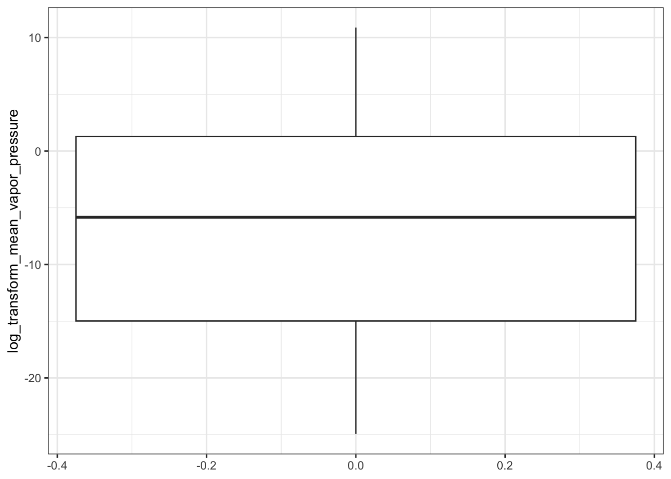
ggplot(ccl4_vapor_grouped, aes(propType, log_transform_mean_vapor_pressure)) +
  geom_boxplot()
#> Warning: Removed 9 rows containing non-finite outside the scale range (`stat_boxplot()`).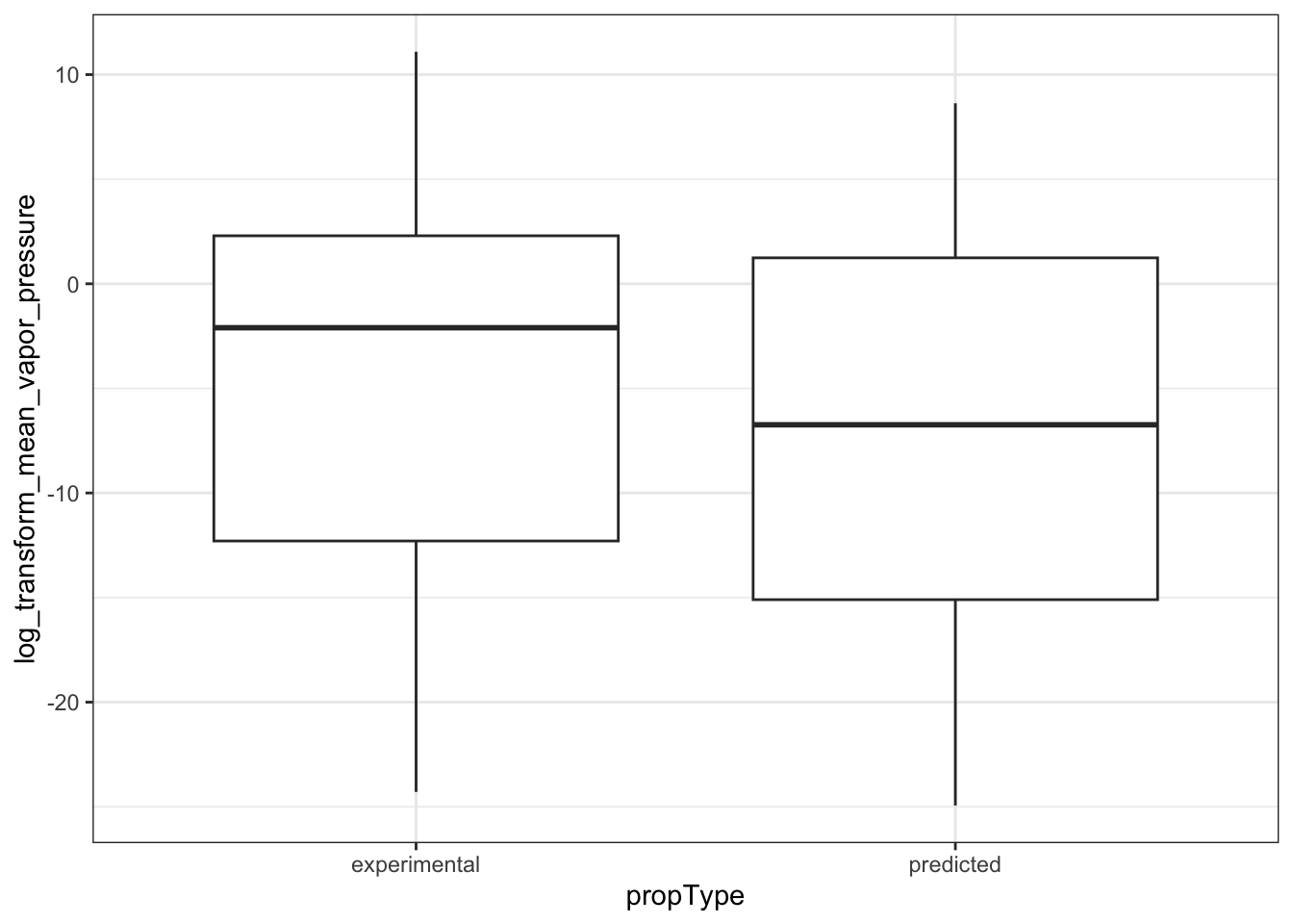
Then plot the NATA data.
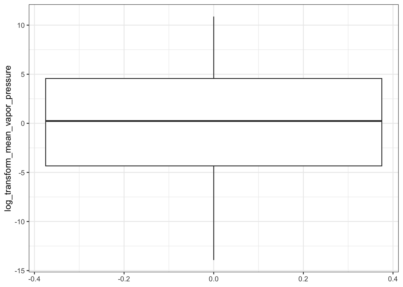
ggplot(natadb_vapor_grouped, aes(propType, log_transform_mean_vapor_pressure)) +
  geom_boxplot()
#> Warning: Removed 3 rows containing non-finite outside the scale range (`stat_boxplot()`).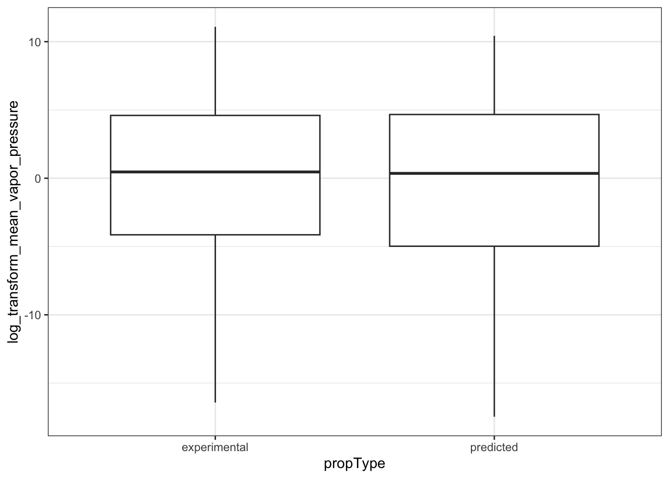
Finally, we compare both sets simultaneously. We add in a column to each data.table denoting to which data set the rows correspond and then combine the rows from both data sets together using the function rbind().
ccl4_vapor_grouped[, set := 'CCL4']
#>             dtxsid     propType mean_vapor_pressure log_transform_mean_vapor_pressure    set
#>             <char>       <char>               <num>                             <num> <char>
#>   1: DTXSID0020153 experimental        1.227658e+00                         0.2051079   CCL4
#>   2: DTXSID0020153    predicted        1.502224e+00                         0.4069466   CCL4
#>   3: DTXSID0020446 experimental        1.878700e-07                       -15.4875156   CCL4
#>   4: DTXSID0020446    predicted        1.592261e-06                       -13.3503554   CCL4
#>   5: DTXSID0020573 experimental        2.825234e-11                       -24.2898450   CCL4
#>  ---
#> 170: DTXSID9032113 experimental        1.301896e-08                       -18.1568589   CCL4
#> 171: DTXSID9032113    predicted        3.547356e-08                       -17.1544782   CCL4
#> 172: DTXSID9032119    predicted                 NaN                               NaN   CCL4
#> 173: DTXSID9032329 experimental        8.494045e-07                       -13.9787303   CCL4
#> 174: DTXSID9032329    predicted        6.692655e-07                       -14.2170850   CCL4
natadb_vapor_grouped[, set := 'NATADB']
#>             dtxsid     propType mean_vapor_pressure log_transform_mean_vapor_pressure    set
#>             <char>       <char>               <num>                             <num> <char>
#>   1: DTXSID0020153 experimental        1.227658e+00                         0.2051079 NATADB
#>   2: DTXSID0020153    predicted        1.502224e+00                         0.4069466 NATADB
#>   3: DTXSID0020448 experimental        5.663676e+01                         4.0366582 NATADB
#>   4: DTXSID0020448    predicted        4.764624e+01                         3.8638038 NATADB
#>   5: DTXSID0020523 experimental        2.446884e-04                        -8.3155250 NATADB
#>  ---
#> 300: DTXSID9021138 experimental        3.359335e-03                        -5.6960121 NATADB
#> 301: DTXSID9021138    predicted        3.622429e-03                        -5.6206104 NATADB
#> 302: DTXSID9021261 experimental        7.500620e-04                        -7.1953547 NATADB
#> 303: DTXSID9021261    predicted                 NaN                               NaN NATADB
#> 304: DTXSID9041522    predicted        6.434033e-05                        -9.6513239 NATADB

all_vapor_grouped <- rbind(ccl4_vapor_grouped, natadb_vapor_grouped)
Now we plot the combined data. First we color the boxplots based on the property type, with mean log transformed vapor pressure plotted for each data set and property type.
vapor_box <- ggplot(all_vapor_grouped,
                    aes(set, log_transform_mean_vapor_pressure)) +
  geom_boxplot(aes(color = propType))
vapor_box
#> Warning: Removed 12 rows containing non-finite outside the scale range (`stat_boxplot()`).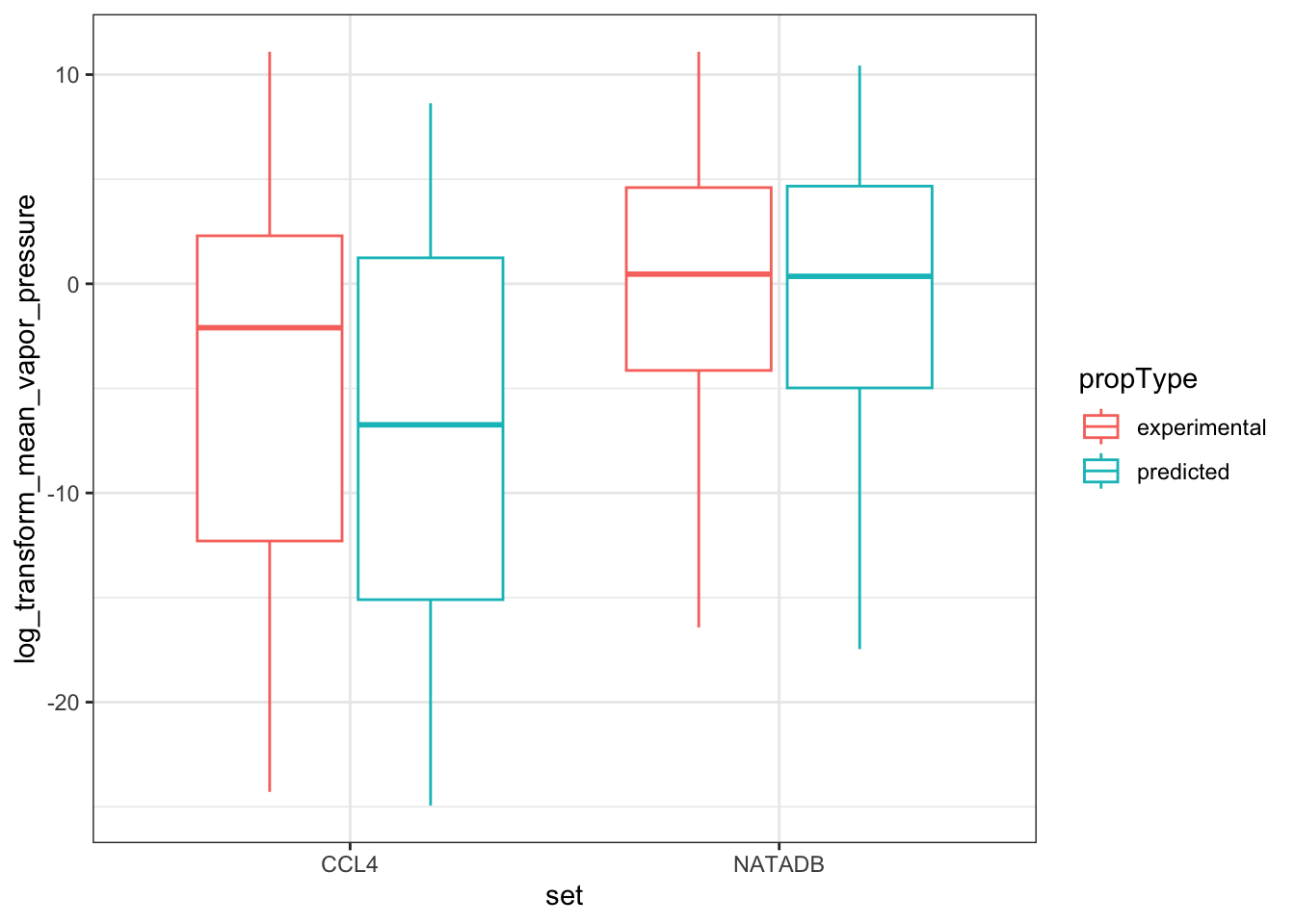
Next we color the boxplots based on the data set.
vapor <- ggplot(all_vapor_grouped, aes(log_transform_mean_vapor_pressure)) +
  geom_boxplot((aes(color = set))) +
  coord_flip()
vapor
#> Warning: Removed 12 rows containing non-finite outside the scale range (`stat_boxplot()`).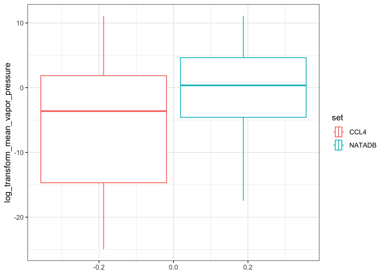
In the plots above, when we graph the data separated both by data set and property type as well as just by data set, we observe the general trend that the NATADB chemicals have a higher mean vapor pressure than the CCL4 chemicals.
We also explore Henry’s Law constant and boiling point in a similar fashion.
Group by DTXSID.
ccl4_hlc_all <- ccl4_phys_chem[propName %in% "Henry's Law Constant",
                               .(mean_hlc = sapply(.SD, function(t) {mean(t, na.rm = TRUE)})),
                               .SDcols = c('propValue'), by = .(dtxsid)]
natadb_hlc_all <- natadb_phys_chem[propName %in% "Henry's Law Constant",
                                   .(mean_hlc = sapply(.SD, function(t) {mean(t, na.rm = TRUE)})),
                                   .SDcols = c('propValue'), by = .(dtxsid)]
Group by DTXSID and property type.
ccl4_hlc_grouped <- ccl4_phys_chem[propName %in% "Henry's Law Constant",
                                   .(mean_hlc = sapply(.SD, function(t) {mean(t, na.rm = TRUE)})),
                                   .SDcols = c('propValue'),
                                   by = .(dtxsid, propType)]
natadb_hlc_grouped <- natadb_phys_chem[propName %in% "Henry's Law Constant",
                                       .(mean_hlc = sapply(.SD, function(t) {mean(t, na.rm = TRUE)})),
                                       .SDcols = c('propValue'),
                                       by = .(dtxsid, propType)]
Examine summary statistics.
summary(ccl4_hlc_all)
#>     dtxsid             mean_hlc
#>  Length:90          Min.   :0.000e+00
#>  Class :character   1st Qu.:1.000e-08
#>  Mode  :character   Median :1.100e-06
#>                     Mean   :2.102e-02
#>                     3rd Qu.:9.665e-05
#>                     Max.   :1.501e+00
summary(ccl4_hlc_grouped)
#>     dtxsid            propType            mean_hlc
#>  Length:157         Length:157         Min.   :0.000e+00
#>  Class :character   Class :character   1st Qu.:1.000e-08
#>  Mode  :character   Mode  :character   Median :1.460e-06
#>                                        Mean   :1.667e-02
#>                                        3rd Qu.:1.291e-04
#>                                        Max.   :1.547e+00
#>                                        NA's   :2
summary(natadb_hlc_all)
#>     dtxsid             mean_hlc
#>  Length:152         Min.   :   0.0000
#>  Class :character   1st Qu.:   0.0000
#>  Mode  :character   Median :   0.0001
#>                     Mean   :  25.1947
#>                     3rd Qu.:   0.0024
#>                     Max.   :3824.2932
summary(natadb_hlc_grouped)
#>     dtxsid            propType            mean_hlc
#>  Length:274         Length:274         Min.   :   0.0000
#>  Class :character   Class :character   1st Qu.:   0.0000
#>  Mode  :character   Mode  :character   Median :   0.0001
#>                                        Mean   :  14.8546
#>                                        3rd Qu.:   0.0024
#>                                        Max.   :4063.3114
Again, we log transform the data as it covers several orders of magnitude. We expect these values to be positive in general so we go ahead with these transformations.
ccl4_hlc_all[, log_transform_mean_hlc := log(mean_hlc)]
#>             dtxsid     mean_hlc log_transform_mean_hlc
#>             <char>        <num>                  <num>
#>  1:  DTXSID0020153 7.608625e-04             -7.1810579
#>  2:  DTXSID0020446 5.917914e-08            -16.6426967
#>  3:  DTXSID0020573 3.715352e-06            -12.5030371
#>  4:  DTXSID0020600 1.493028e-04             -8.8095341
#>  5:  DTXSID0020814 2.041738e-07            -15.4042943
#>  6:  DTXSID0021464 1.678272e-08            -17.9029160
#>  7:  DTXSID0021541 9.965029e-03             -4.6086735
#>  8:  DTXSID0021917 1.501363e+00              0.4063731
#>  9:  DTXSID0024052 9.335794e-11            -23.0945802
#> 10:  DTXSID0032578 5.708485e-07            -14.3761419
#> 11:  DTXSID1020437 5.910373e-03             -5.1310463
#> 12:  DTXSID1021407 9.105946e-07            -13.9091681
#> 13:  DTXSID1021409 4.290971e-07            -14.6615827
#> 14:  DTXSID1021740 1.284597e-05            -11.2624803
#> 15:  DTXSID1021798 2.071620e-06            -13.0871795
#> 16:  DTXSID1024174 1.509734e-06            -13.4035773
#> 17:  DTXSID1024338 3.665514e-09            -19.4242972
#> 18:  DTXSID1026164 1.978642e-06            -13.1330997
#> 19:  DTXSID1037484 1.202264e-09            -20.5390590
#> 20:  DTXSID1037486 1.174898e-09            -20.5620849
#> 21:  DTXSID1037567 4.365158e-10            -21.5521965
#> 22:  DTXSID2020684 8.526210e-06            -11.6723656
#> 23:  DTXSID2021028 1.677186e-04             -8.6932227
#> 24:  DTXSID2021317 2.391691e-03             -6.0357547
#> 25:  DTXSID2021731 1.585469e-05            -11.0520451
#> 26:  DTXSID2022333 1.488889e-02             -4.2071400
#> 27:  DTXSID2031083 5.623413e-11            -23.6014972
#> 28:  DTXSID2037506 3.176631e-09            -19.5674445
#> 29:  DTXSID2052156 3.801894e-10            -21.6903516
#> 30:  DTXSID3020203 2.795640e-01             -1.2745241
#> 31:  DTXSID3020702 6.168270e-07            -14.2986772
#> 32:  DTXSID3020833 6.305823e-04             -7.3688669
#> 33:  DTXSID3020964 4.483844e-05            -10.0124448
#> 34:  DTXSID3021857 2.089296e-03             -6.1709280
#> 35:  DTXSID3024366 1.476024e-04             -8.8209882
#> 36:  DTXSID3024869 6.240907e-07            -14.2869701
#> 37:  DTXSID3031864 1.819701e-11            -24.7297639
#> 38:  DTXSID3032464 2.241663e-06            -13.0082925
#> 39:  DTXSID3034458 8.128305e-09            -18.6279134
#> 40:  DTXSID3042219 1.016034e-02             -4.5892630
#> 41:  DTXSID3074313 2.041738e-11            -24.6146346
#> 42:  DTXSID4020533 5.273916e-06            -12.1527374
#> 43:  DTXSID4021503 1.902843e-03             -6.2644060
#> 44:  DTXSID4022361 3.267786e-08            -17.2365681
#> 45:  DTXSID4022367 1.047129e-09            -20.6772141
#> 46:  DTXSID4022448 2.132508e-08            -17.6633821
#> 47:  DTXSID4022991 1.230269e-11            -25.1212034
#> 48:  DTXSID4032611 3.812004e-06            -12.4773554
#> 49:  DTXSID4034948 5.061593e-09            -19.1015846
#> 50:  DTXSID5020023 1.844509e-04             -8.5981272
#> 51:  DTXSID5020576 9.332543e-08            -16.1871732
#> 52:  DTXSID5020601 2.032776e-07            -15.4086934
#> 53:  DTXSID5021207 8.762638e-05             -9.3424285
#> 54:  DTXSID5024182 7.477348e-03             -4.8958771
#> 55:  DTXSID5039224 7.530076e-05             -9.4940203
#> 56: DTXSID50867064 1.174898e-08            -18.2594998
#> 57:  DTXSID6020301 3.266831e-02             -3.4213498
#> 58:  DTXSID6020856 4.568074e-04             -7.6912486
#> 59:  DTXSID6021030 7.565670e-04             -7.1867194
#> 60:  DTXSID6021032 8.403150e-05             -9.3843188
#> 61:  DTXSID6022422 5.360194e-08            -16.7416806
#> 62:  DTXSID6024177 1.285277e-07            -15.8671213
#> 63:  DTXSID6037483 5.495409e-10            -21.3219380
#> 64:  DTXSID6037485 5.623413e-10            -21.2989121
#> 65:  DTXSID6037568 8.317638e-09            -18.6048876
#> 66:  DTXSID7020005 2.450917e-08            -17.5242187
#> 67:  DTXSID7020637 4.882250e-07            -14.5324894
#> 68:  DTXSID7021029 1.281830e-05            -11.2646365
#> 69:  DTXSID7024241 1.297787e-06            -13.5548503
#> 70:  DTXSID7047433 6.760830e-08            -16.5095351
#> 71:  DTXSID8020044 4.981622e-06            -12.2097550
#> 72:  DTXSID8020090 7.725040e-03             -4.8632882
#> 73:  DTXSID8020597 2.350772e-07            -15.2633520
#> 74:  DTXSID8020832 1.144615e-02             -4.4701020
#> 75:  DTXSID8021062 3.866425e-06            -12.4631803
#> 76:  DTXSID8022292 1.451240e-06            -13.4430924
#> 77:  DTXSID8022377 3.715352e-06            -12.5030371
#> 78:  DTXSID8023846 1.632925e-09            -20.2328929
#> 79:  DTXSID8023848 1.032272e-08            -18.3889189
#> 80:  DTXSID8025541 4.168694e-07            -14.6904929
#> 81:  DTXSID8031865 9.965663e-05             -9.2137800
#> 82:  DTXSID9020243 1.907474e-06            -13.1697307
#> 83:  DTXSID9021390 3.108242e-04             -8.0762831
#> 84:  DTXSID9021427 2.270435e-07            -15.2981240
#> 85:  DTXSID9022366 5.128614e-09            -19.0884304
#> 86:  DTXSID9023380 4.168694e-09            -19.2956631
#> 87:  DTXSID9023914 5.003672e-11            -23.7182639
#> 88:  DTXSID9024142 1.345777e-06            -13.5185387
#> 89:  DTXSID9032113 7.734149e-08            -16.3750352
#> 90:  DTXSID9032329 5.382367e-07            -14.4349674
#>             dtxsid     mean_hlc log_transform_mean_hlc
#>             <char>        <num>                  <num>
ccl4_hlc_grouped[, log_transform_mean_hlc := log(mean_hlc)]
#>             dtxsid     propType     mean_hlc log_transform_mean_hlc
#>             <char>       <char>        <num>                  <num>
#>   1: DTXSID0020153 experimental 4.870692e-04              -7.627104
#>   2: DTXSID0020153    predicted 2.951209e-03              -5.825540
#>   3: DTXSID0020446 experimental 7.359553e-08             -16.424682
#>   4: DTXSID0020446    predicted 1.513561e-09             -20.308801
#>   5: DTXSID0020573    predicted 3.715352e-06             -12.503037
#>  ---
#> 153: DTXSID9024142    predicted 2.691535e-06             -12.825399
#> 154: DTXSID9032113 experimental 1.121455e-10             -22.911224
#> 155: DTXSID9032113    predicted 3.090295e-07             -14.989829
#> 156: DTXSID9032329 experimental 1.490847e-08             -18.021336
#> 157: DTXSID9032329    predicted 1.584893e-06             -13.354994

natadb_hlc_all[, log_transform_mean_hlc := log(mean_hlc)]
#>             dtxsid     mean_hlc log_transform_mean_hlc
#>             <char>        <num>                  <num>
#>   1: DTXSID0020153 7.608625e-04              -7.181058
#>   2: DTXSID0020448 2.710185e-03              -5.910739
#>   3: DTXSID0020523 1.068282e-07             -16.052044
#>   4: DTXSID0020529 2.793630e-07             -15.090754
#>   5: DTXSID0020600 1.493028e-04              -8.809534
#>  ---
#> 148: DTXSID9020293 2.951209e-06             -12.733296
#> 149: DTXSID9020299 9.828547e-08             -16.135390
#> 150: DTXSID9020827 1.813010e-06             -13.220522
#> 151: DTXSID9021138 5.623413e-08             -16.693742
#> 152: DTXSID9041522 8.912509e-06             -11.628055
natadb_hlc_grouped[, log_transform_mean_hlc := log(mean_hlc)]
#>             dtxsid     propType     mean_hlc log_transform_mean_hlc
#>             <char>       <char>        <num>                  <num>
#>   1: DTXSID0020153 experimental 4.870692e-04              -7.627104
#>   2: DTXSID0020153    predicted 2.951209e-03              -5.825540
#>   3: DTXSID0020448 experimental 2.707002e-03              -5.911913
#>   4: DTXSID0020448    predicted 2.818383e-03              -5.871592
#>   5: DTXSID0020523 experimental 1.107746e-07             -16.015769
#>  ---
#> 270: DTXSID9020299    predicted 4.897788e-10             -21.437067
#> 271: DTXSID9020827 experimental 2.134778e-06             -13.057148
#> 272: DTXSID9020827    predicted 2.041738e-07             -15.404294
#> 273: DTXSID9021138    predicted 5.623413e-08             -16.693742
#> 274: DTXSID9041522    predicted 8.912509e-06             -11.628055
We compare both sets simultaneously. We add in a column to each data.table denoting to which set the rows correspond and then rbind() the rows together.
Label and combine data.
ccl4_hlc_grouped[, set := 'CCL4']
#>             dtxsid     propType     mean_hlc log_transform_mean_hlc    set
#>             <char>       <char>        <num>                  <num> <char>
#>   1: DTXSID0020153 experimental 4.870692e-04              -7.627104   CCL4
#>   2: DTXSID0020153    predicted 2.951209e-03              -5.825540   CCL4
#>   3: DTXSID0020446 experimental 7.359553e-08             -16.424682   CCL4
#>   4: DTXSID0020446    predicted 1.513561e-09             -20.308801   CCL4
#>   5: DTXSID0020573    predicted 3.715352e-06             -12.503037   CCL4
#>  ---
#> 153: DTXSID9024142    predicted 2.691535e-06             -12.825399   CCL4
#> 154: DTXSID9032113 experimental 1.121455e-10             -22.911224   CCL4
#> 155: DTXSID9032113    predicted 3.090295e-07             -14.989829   CCL4
#> 156: DTXSID9032329 experimental 1.490847e-08             -18.021336   CCL4
#> 157: DTXSID9032329    predicted 1.584893e-06             -13.354994   CCL4
natadb_hlc_grouped[, set := 'NATADB']
#>             dtxsid     propType     mean_hlc log_transform_mean_hlc    set
#>             <char>       <char>        <num>                  <num> <char>
#>   1: DTXSID0020153 experimental 4.870692e-04              -7.627104 NATADB
#>   2: DTXSID0020153    predicted 2.951209e-03              -5.825540 NATADB
#>   3: DTXSID0020448 experimental 2.707002e-03              -5.911913 NATADB
#>   4: DTXSID0020448    predicted 2.818383e-03              -5.871592 NATADB
#>   5: DTXSID0020523 experimental 1.107746e-07             -16.015769 NATADB
#>  ---
#> 270: DTXSID9020299    predicted 4.897788e-10             -21.437067 NATADB
#> 271: DTXSID9020827 experimental 2.134778e-06             -13.057148 NATADB
#> 272: DTXSID9020827    predicted 2.041738e-07             -15.404294 NATADB
#> 273: DTXSID9021138    predicted 5.623413e-08             -16.693742 NATADB
#> 274: DTXSID9041522    predicted 8.912509e-06             -11.628055 NATADB

all_hlc_grouped <- rbind(ccl4_hlc_grouped, natadb_hlc_grouped)
Plot data. Some rows are removed due to transformations above that result in non-valid values.
hlc_box <- ggplot(all_hlc_grouped, aes(set, log_transform_mean_hlc)) +
  geom_boxplot(aes(color = propType))
hlc_box
#> Warning: Removed 2 rows containing non-finite outside the scale range (`stat_boxplot()`).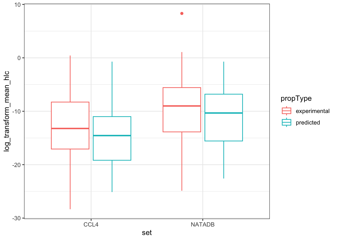
hlc <- ggplot(all_hlc_grouped, aes(log_transform_mean_hlc)) +
  geom_boxplot(aes(color = set)) +
  coord_flip()
hlc
#> Warning: Removed 2 rows containing non-finite outside the scale range (`stat_boxplot()`).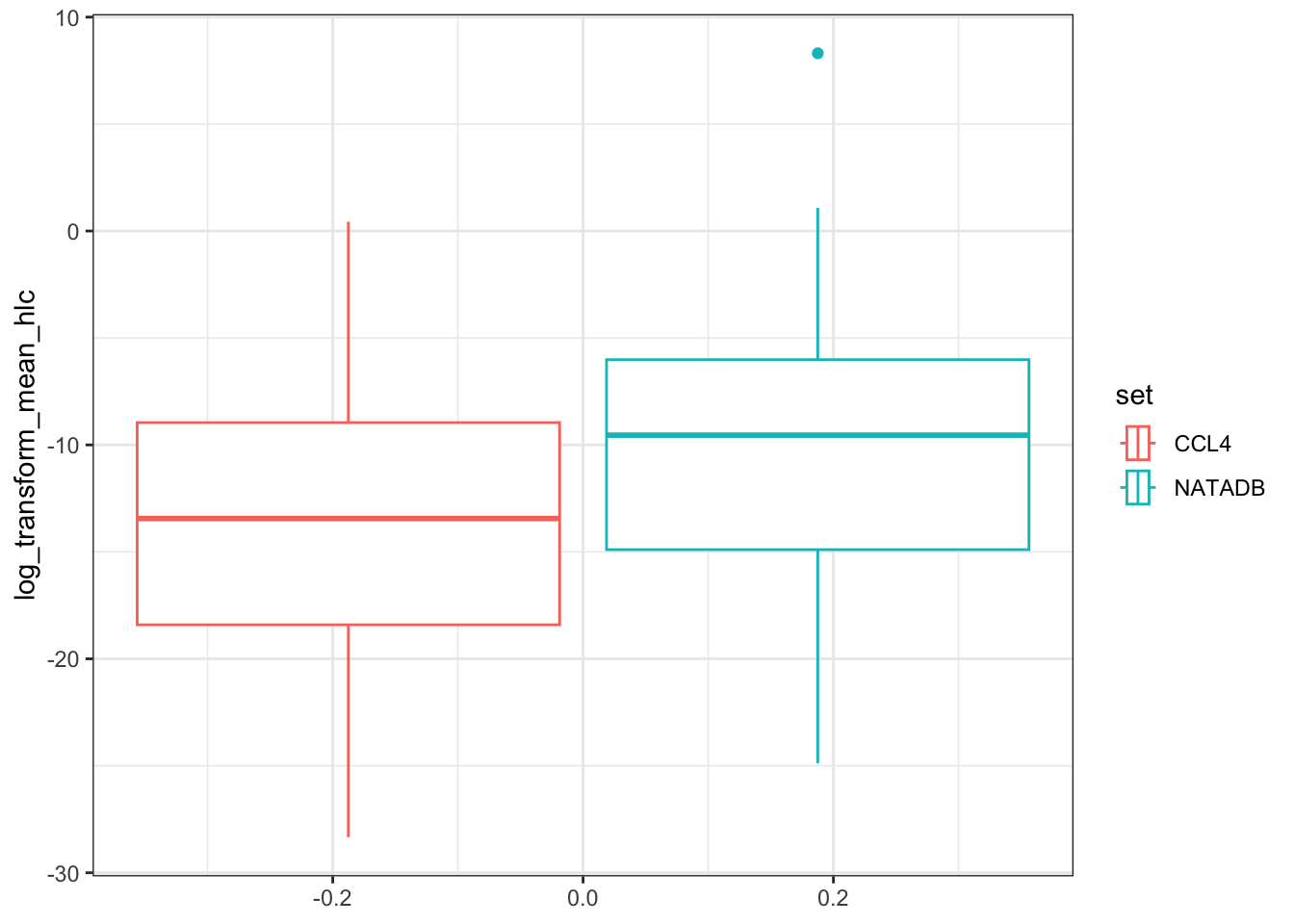
Again, we observe that in both grouping by propType and aggregating all results together by data set, that the chemicals in NATADB have a generally higher mean Henry’s Law Constant value than those in CCL4.
Finally, we consider boiling point.
Group by DTXSID.
ccl4_boiling_all <- ccl4_phys_chem[propName %in% 'Boiling Point',
                                   .(mean_boiling_point = sapply(.SD, function(t) {mean(t, na.rm = TRUE)})),
                                   .SDcols = c('propValue'), by = .(dtxsid)]
natadb_boiling_all <- natadb_phys_chem[propName %in% 'Boiling Point',
                                       .(mean_boiling_point =
                                           sapply(.SD, function(t) {mean(t, na.rm = TRUE)})),
                                       .SDcols = c('propValue'), by = .(dtxsid)]
Group by DTXSID and property type.
ccl4_boiling_grouped <- ccl4_phys_chem[propName %in% 'Boiling Point',
                                       .(mean_boiling_point =
                                           sapply(.SD, function(t) {mean(t, na.rm = TRUE)})),
                                       .SDcols = c('propValue'),
                                       by = .(dtxsid, propType)]
natadb_boiling_grouped <- natadb_phys_chem[propName %in% 'Boiling Point',
                                           .(mean_boiling_point =
                                               sapply(.SD, function(t) {mean(t, na.rm = TRUE)})),
                                           .SDcols = c('propValue'),
                                           by = .(dtxsid, propType)]
Calculate summary statistics.
summary(ccl4_boiling_all)
#>     dtxsid          mean_boiling_point
#>  Length:99          Min.   : -37.75
#>  Class :character   1st Qu.: 173.91
#>  Mode  :character   Median : 268.00
#>                     Mean   : 372.73
#>                     3rd Qu.: 378.49
#>                     Max.   :4745.20
#>                     NA's   :2
summary(ccl4_boiling_grouped)
#>     dtxsid            propType         mean_boiling_point
#>  Length:158         Length:158         Min.   : -40.71
#>  Class :character   Class :character   1st Qu.: 117.84
#>  Mode  :character   Mode  :character   Median : 210.00
#>                                        Mean   : 298.89
#>                                        3rd Qu.: 348.13
#>                                        Max.   :4745.20
#>                                        NA's   :7
summary(natadb_boiling_all)
#>     dtxsid          mean_boiling_point
#>  Length:155         Min.   :-87.60
#>  Class :character   1st Qu.: 79.91
#>  Mode  :character   Median :181.46
#>                     Mean   :178.28
#>                     3rd Qu.:266.80
#>                     Max.   :685.00
summary(natadb_boiling_grouped)
#>     dtxsid            propType         mean_boiling_point
#>  Length:298         Length:298         Min.   :-87.64
#>  Class :character   Class :character   1st Qu.: 76.61
#>  Mode  :character   Mode  :character   Median :177.59
#>                                        Mean   :171.41
#>                                        3rd Qu.:255.68
#>                                        Max.   :685.00
#>                                        NA's   :3
Since some of the boiling point values have negative values, we cannot log transform these values. If we try, as you will see below, there will be warnings of NaNs produced.
ccl4_boiling_all[, log_transform := log(mean_boiling_point)]
#> Warning in log(mean_boiling_point): NaNs produced
#>             dtxsid mean_boiling_point log_transform
#>             <char>              <num>         <num>
#>  1:  DTXSID0020153         178.578246      5.185027
#>  2:  DTXSID0020446         309.446204      5.734784
#>  3:  DTXSID0020573         402.793157      5.998423
#>  4:  DTXSID0020600          12.425270      2.519732
#>  5:  DTXSID0020814         394.526706      5.977687
#>  6:  DTXSID0021464         177.000000      5.176150
#>  7:  DTXSID0021541         -21.764660           NaN
#>  8:  DTXSID0021917          69.123815      4.235899
#>  9:  DTXSID0024052         386.788500      5.957878
#> 10:  DTXSID0024341         193.018519      5.262786
#> 11:  DTXSID0032578         382.420000      5.946519
#> 12:  DTXSID1020437          57.462613      4.051135
#> 13:  DTXSID1021407         247.544453      5.511590
#> 14:  DTXSID1021409         428.540000      6.060384
#> 15:  DTXSID1021740         117.737019      4.768453
#> 16:  DTXSID1021798         237.494012      5.470142
#> 17:  DTXSID1024174         320.600667      5.770196
#> 18:  DTXSID1024207        4745.200000      8.464889
#> 19:  DTXSID1024338         265.000000      5.579730
#> 20:  DTXSID1026164         202.214627      5.309330
#> 21:  DTXSID1031040        2870.000000      7.962067
#> 22:  DTXSID1037484         359.716089      5.885315
#> 23:  DTXSID1037486         360.471401      5.887413
#> 24:  DTXSID1037567         359.067259      5.883510
#> 25:  DTXSID2020684         272.058098      5.606016
#> 26:  DTXSID2021028         177.407265      5.178448
#> 27:  DTXSID2021317         130.561056      4.871841
#> 28:  DTXSID2021731          68.940190      4.233239
#> 29:  DTXSID2022333         173.914044      5.158561
#> 30:  DTXSID2024169        1962.111111      7.581776
#> 31:  DTXSID2031083         265.000000      5.579730
#> 32:  DTXSID2037506         322.058999      5.774735
#> 33:  DTXSID2040282                NaN           NaN
#> 34:  DTXSID2052156         413.356503      6.024310
#> 35:  DTXSID3020203          -2.284146           NaN
#> 36:  DTXSID3020702         115.631944      4.750412
#> 37:  DTXSID3020833          56.744806      4.038564
#> 38:  DTXSID3020964         210.912673      5.351444
#> 39:  DTXSID3021857         281.000000      5.638355
#> 40:  DTXSID3024366          88.996924      4.488602
#> 41:  DTXSID3024869         207.710000      5.336143
#> 42:  DTXSID3031864         242.988116      5.493013
#> 43:  DTXSID3032464         382.914500      5.947812
#> 44:  DTXSID3034458         404.806000      6.003408
#> 45:  DTXSID3042219         160.235980      5.076648
#> 46:  DTXSID3073137                NaN           NaN
#> 47:  DTXSID3074313         423.281500      6.048037
#> 48:  DTXSID4020533         101.194672      4.617046
#> 49:  DTXSID4021503          67.649123      4.214334
#> 50:  DTXSID4022361         362.481861      5.892974
#> 51:  DTXSID4022367         384.354700      5.951566
#> 52:  DTXSID4022448         343.803404      5.840070
#> 53:  DTXSID4022991         588.505984      6.377587
#> 54:  DTXSID4032611         280.169000      5.635393
#> 55:  DTXSID4034948         329.000000      5.796058
#> 56:  DTXSID5020023          52.663575      3.963924
#> 57:  DTXSID5020576         410.106570      6.016417
#> 58:  DTXSID5020601         303.273281      5.714634
#> 59:  DTXSID5021207          36.671712      3.602006
#> 60:  DTXSID5024182         124.424454      4.823699
#> 61:  DTXSID5039224          21.121067      3.050271
#> 62: DTXSID50867064         263.260860      5.573145
#> 63:  DTXSID6020301         -37.747068           NaN
#> 64:  DTXSID6020856         201.604415      5.306307
#> 65:  DTXSID6021030         230.209089      5.438988
#> 66:  DTXSID6021032         207.304345      5.334188
#> 67:  DTXSID6022422         396.072602      5.981598
#> 68:  DTXSID6024177         223.850000      5.410976
#> 69:  DTXSID6037483         348.558155      5.853805
#> 70:  DTXSID6037485         347.701654      5.851345
#> 71:  DTXSID6037568         362.244245      5.892319
#> 72:  DTXSID7020005         213.701630      5.364581
#> 73:  DTXSID7020215         268.000000      5.590987
#> 74:  DTXSID7020637         -10.271938           NaN
#> 75:  DTXSID7021029         153.627548      5.034531
#> 76:  DTXSID7024241         365.692761      5.901794
#> 77:  DTXSID7047433         391.174129      5.969153
#> 78:  DTXSID8020044          95.670634      4.560911
#> 79:  DTXSID8020090         184.656010      5.218495
#> 80:  DTXSID8020597         192.848532      5.261905
#> 81:  DTXSID8020832           4.547273      1.514528
#> 82:  DTXSID8021062         212.429837      5.358612
#> 83:  DTXSID8022292         369.819083      5.913014
#> 84:  DTXSID8022377         399.240876      5.989565
#> 85:  DTXSID8023846         287.000000      5.659482
#> 86:  DTXSID8023848         300.446797      5.705271
#> 87:  DTXSID8025541         339.798000      5.828351
#> 88:  DTXSID8031865         190.626163      5.250314
#> 89:  DTXSID8052483        2700.000000      7.901007
#> 90:  DTXSID9020243         308.081500      5.730364
#> 91:  DTXSID9021390         155.399500      5.045999
#> 92:  DTXSID9021427         182.970974      5.209328
#> 93:  DTXSID9022366         414.696312      6.027546
#> 94:  DTXSID9023380         378.489580      5.936189
#> 95:  DTXSID9023914         359.534841      5.884811
#> 96:  DTXSID9024142         427.009000      6.056805
#> 97:  DTXSID9032113         381.238490      5.943425
#> 98:  DTXSID9032119        1089.950000      6.993887
#> 99:  DTXSID9032329         436.091500      6.077852
#>             dtxsid mean_boiling_point log_transform
#>             <char>              <num>         <num>
ccl4_boiling_grouped[, log_transform := log(mean_boiling_point)]
#> Warning in log(mean_boiling_point): NaNs produced
#>             dtxsid     propType mean_boiling_point log_transform
#>             <char>       <char>              <num>         <num>
#>   1: DTXSID0020153 experimental           178.4519      5.184319
#>   2: DTXSID0020153    predicted           178.9574      5.187148
#>   3: DTXSID0020446 experimental           270.5000      5.600272
#>   4: DTXSID0020446    predicted           335.4103      5.815355
#>   5: DTXSID0020573 experimental           413.4500      6.024537
#>  ---
#> 154: DTXSID9024142    predicted           501.5135      6.217631
#> 155: DTXSID9032113    predicted           381.2385      5.943425
#> 156: DTXSID9032119 experimental          1089.9500      6.993887
#> 157: DTXSID9032119    predicted                NaN           NaN
#> 158: DTXSID9032329    predicted           436.0915      6.077852

natadb_boiling_all[, log_transform := log(mean_boiling_point)]
#> Warning in log(mean_boiling_point): NaNs produced
#>             dtxsid mean_boiling_point log_transform
#>             <char>              <num>         <num>
#>   1: DTXSID0020153          178.57825      5.185027
#>   2: DTXSID0020448           96.11380      4.565533
#>   3: DTXSID0020523          329.20847      5.796691
#>   4: DTXSID0020529          300.77573      5.706365
#>   5: DTXSID0020600           12.42527      2.519732
#>  ---
#> 151: DTXSID9020299          393.19798      5.974313
#> 152: DTXSID9020827          371.68218      5.918039
#> 153: DTXSID9021138          267.65926      5.589715
#> 154: DTXSID9021261          685.00000      6.529419
#> 155: DTXSID9041522          337.07591      5.820308
natadb_boiling_grouped[, log_transform := log(mean_boiling_point)]
#> Warning in log(mean_boiling_point): NaNs produced
#>             dtxsid     propType mean_boiling_point log_transform
#>             <char>       <char>              <num>         <num>
#>   1: DTXSID0020153 experimental          178.45185      5.184319
#>   2: DTXSID0020153    predicted          178.95743      5.187148
#>   3: DTXSID0020448 experimental           96.07302      4.565108
#>   4: DTXSID0020448    predicted           96.30413      4.567511
#>   5: DTXSID0020523    predicted          329.20847      5.796691
#>  ---
#> 294: DTXSID9021138    predicted          266.71606      5.586185
#> 295: DTXSID9021261 experimental          685.00000      6.529419
#> 296: DTXSID9021261    predicted                NaN           NaN
#> 297: DTXSID9041522 experimental          340.00000      5.828946
#> 298: DTXSID9041522    predicted          332.20241      5.805744
We compare both sets simultaneously. We add in a column to each data.table denoting to which set the rows correspond and then rbind() the rows together. We use the values as is rather than transforming them.
Label and combine data.
ccl4_boiling_grouped[, set := 'CCL4']
#>             dtxsid     propType mean_boiling_point log_transform    set
#>             <char>       <char>              <num>         <num> <char>
#>   1: DTXSID0020153 experimental           178.4519      5.184319   CCL4
#>   2: DTXSID0020153    predicted           178.9574      5.187148   CCL4
#>   3: DTXSID0020446 experimental           270.5000      5.600272   CCL4
#>   4: DTXSID0020446    predicted           335.4103      5.815355   CCL4
#>   5: DTXSID0020573 experimental           413.4500      6.024537   CCL4
#>  ---
#> 154: DTXSID9024142    predicted           501.5135      6.217631   CCL4
#> 155: DTXSID9032113    predicted           381.2385      5.943425   CCL4
#> 156: DTXSID9032119 experimental          1089.9500      6.993887   CCL4
#> 157: DTXSID9032119    predicted                NaN           NaN   CCL4
#> 158: DTXSID9032329    predicted           436.0915      6.077852   CCL4
natadb_boiling_grouped[, set := 'NATADB']
#>             dtxsid     propType mean_boiling_point log_transform    set
#>             <char>       <char>              <num>         <num> <char>
#>   1: DTXSID0020153 experimental          178.45185      5.184319 NATADB
#>   2: DTXSID0020153    predicted          178.95743      5.187148 NATADB
#>   3: DTXSID0020448 experimental           96.07302      4.565108 NATADB
#>   4: DTXSID0020448    predicted           96.30413      4.567511 NATADB
#>   5: DTXSID0020523    predicted          329.20847      5.796691 NATADB
#>  ---
#> 294: DTXSID9021138    predicted          266.71606      5.586185 NATADB
#> 295: DTXSID9021261 experimental          685.00000      6.529419 NATADB
#> 296: DTXSID9021261    predicted                NaN           NaN NATADB
#> 297: DTXSID9041522 experimental          340.00000      5.828946 NATADB
#> 298: DTXSID9041522    predicted          332.20241      5.805744 NATADB

all_boiling_grouped <- rbind(ccl4_boiling_grouped, natadb_boiling_grouped)
Plot the data.
boiling_box <- ggplot(all_boiling_grouped, aes(set, mean_boiling_point)) +
  geom_boxplot(aes(color = propType))
boiling_box
#> Warning: Removed 10 rows containing non-finite outside the scale range (`stat_boxplot()`).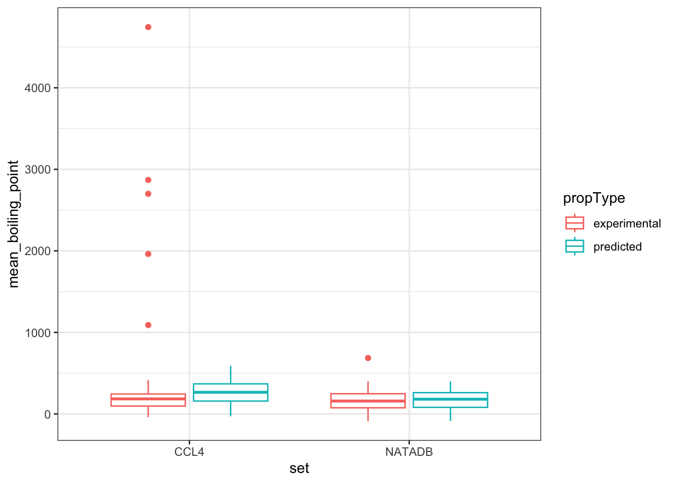
boiling <- ggplot(all_boiling_grouped, aes(mean_boiling_point)) +
  geom_boxplot(aes(color = set)) +
  coord_flip()
boiling
#> Warning: Removed 10 rows containing non-finite outside the scale range (`stat_boxplot()`).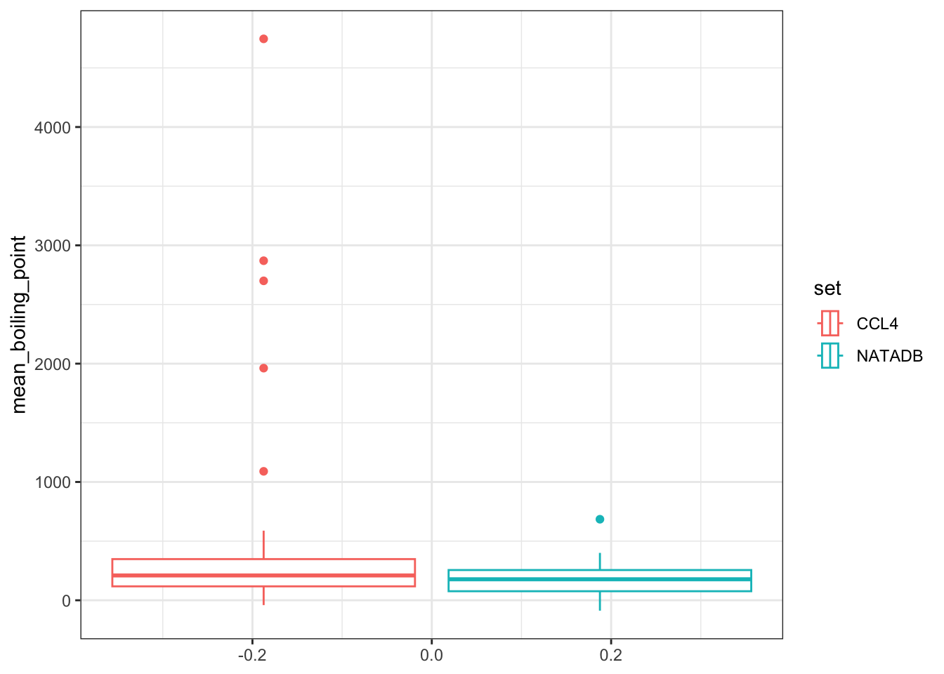
A visual inspection of this set of graphs is not as clear as in the previous cases. Note that the experimental values for each data set tend to be higher than the predicted. The mean of CCL4, by predicted and experimental appears to be greater than the corresponding means for NATADB, as does the overall mean, but the interquartile ranges of these different groupings yield slightly different results. This gives us a sense that the picture for boiling point is not as clear cut between experimental and predicted for these two data sets as it was in the previous cases of physico-chemical properties we investigated.
Answer to Environmental Health Question 2
Through inspecting the last several plots, we can answer Environmental Health Question 2: The physico-chemical property data are reported with both experimental and predicted values present for many chemicals. Are there differences between the mean predicted and experimental results for a variety of physico-chemical properties?
Answer: There are indeed differences between the mean values of various physico-chemical properties when grouped by predicted or experimental. In the case of “Vapor Pressure”, the means of experimental values tend to be a little lower than predicted, though they are much closer in the case of NATADB than CCL4. The trend of lower predicted means compared to experimental means is more clearly demonstrated for “Henry’s Law Constant” values in both data sets. In the case of “Boiling Point”, the experimental values are greater than the predicted values, though this is much more pronounced in CCL4 while the set of means for NATADB are again fairly close.
Hazard Data: Genotoxicity
Now, having examined some of the distributions of the physico-chemical properties of the two lists, aggregated between predicted and experimental, we move towards learning more about these chemicals beyond physico-chemical properties. Specifically, we will examine their genotoxicity.
Using the standard CompTox Chemicals Dashboard approach to access genotoxicity, one would again navigate to the individual chemical page
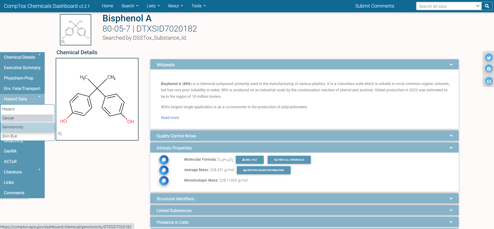
Once one navigates to the genotoxicity tab highlighted in the previous page, the following is displayed as seen here:
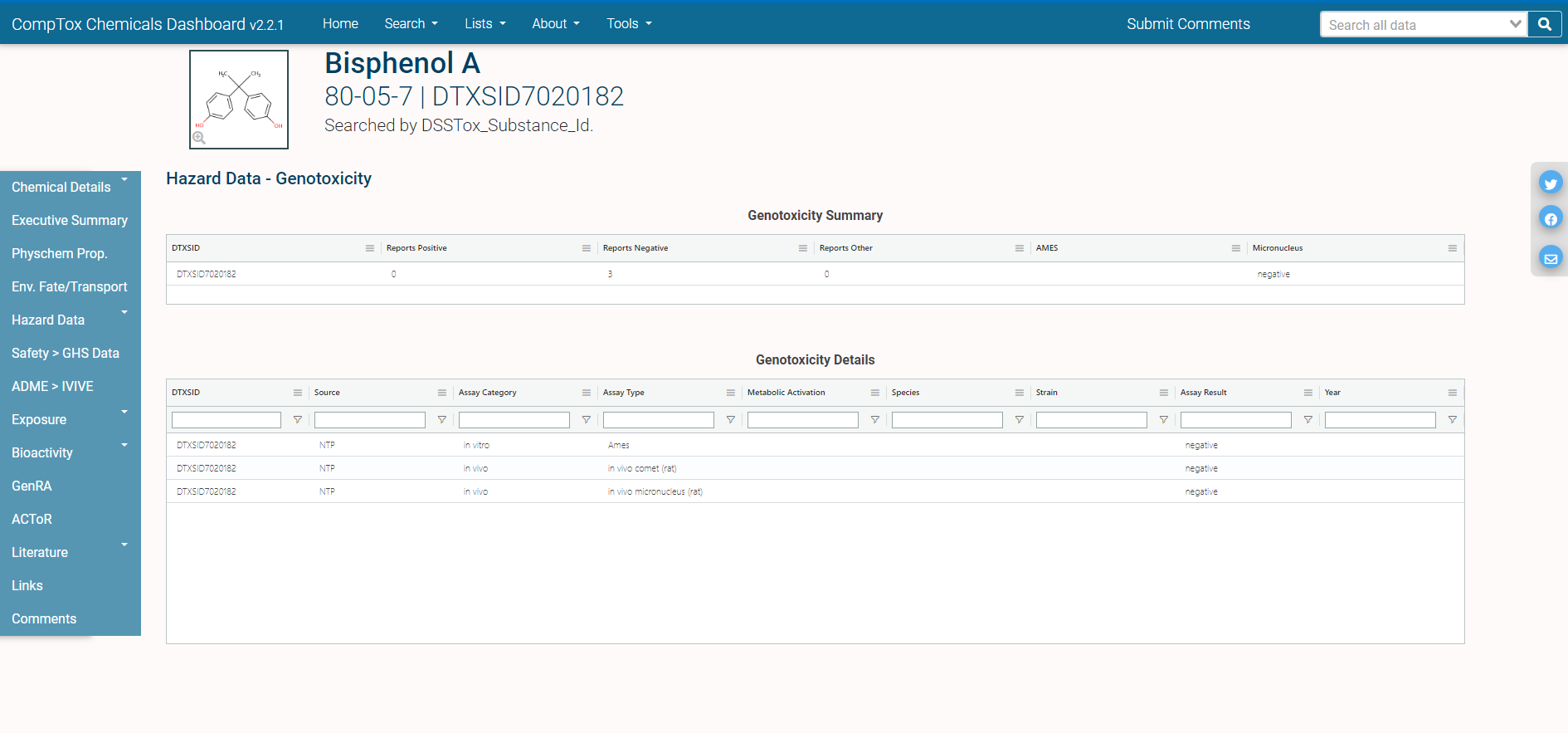
This page includes two sets of information, the first of which provides a summary of available genotoxicity data while the second provides the individual reports and samples of such data.
We again use the CTX APIs to streamline the process of retrieving this information in a programmatic fashion. To this end, we will use the genotoxicity endpoints found within the Hazard endpoints of the CTX APIs. Pictured below is the particular set of genotoxicity resources available in the Hazard endpoints of the CTX APIs.
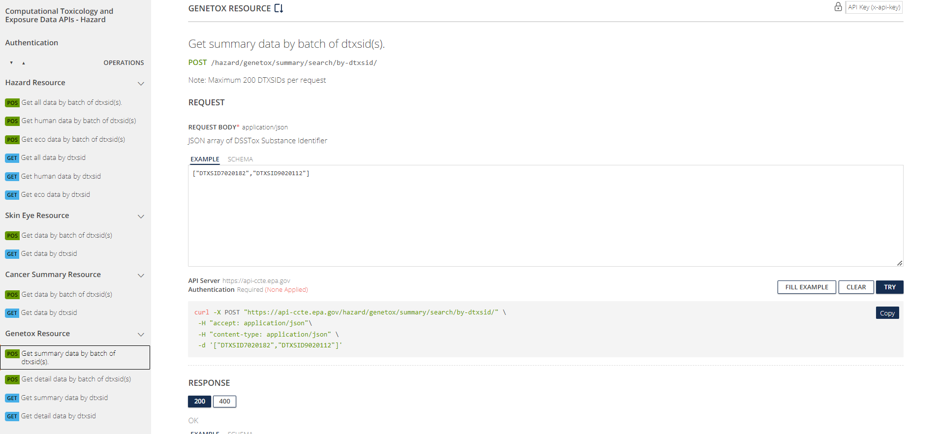
There are both summary and detail resources, reflecting the information one can find on the CompTox Chemicals Dashboard Genotoxicity page for a given chemical.
To access the genetox endpoint, we will use the function get_genetox_summary(). Since we have a list of chemicals, rather than searching individually for each chemical, we use the batch search version of the function, named get_genetox_summary_batch(). We will examine this and then access the details.
Grab the data using the APIs.
ccl4_genotox <- get_genetox_summary_batch(DTXSID = ccl4$dtxsid)
natadb_genetox <- get_genetox_summary_batch(DTXSID = natadb$dtxsid)
Examine the dimensions.
Examine the column names and data from the first six chemicals with genetox data from CCL4.
colnames(ccl4_genotox)
#>  [1] "id"               "dtxsid"           "reportsPositive"  "reportsNegative"  "reportsOther"
#>  [6] "ames"             "micronucleus"     "clowderDocId"     "genetoxCall"      "genetoxSummaryId"
head(ccl4_genotox)
#>       id        dtxsid reportsPositive reportsNegative reportsOther     ames micronucleus
#>    <int>        <char>           <int>           <int>        <int>   <char>       <char>
#> 1:    92 DTXSID0020153              20               5            1 positive     positive
#> 2:  4399 DTXSID0020446               0               8            0 negative     negative
#> 3:   930 DTXSID0020573               3               9            0 negative     negative
#> 4:    93 DTXSID0020600              20               0            1 positive     positive
#> 5:  2079 DTXSID0020814               1               0            0     <NA>         <NA>
#> 6:   320 DTXSID0021464               8               6            0 positive     positive
#> 3 variables not shown: [clowderDocId <char>, genetoxCall <char>, genetoxSummaryId <int>]
The information returned is of the first variety highlighted in the image above, that is, the summary data on the available genotoxicity data for each chemical.
Observe that we have information on 71 chemicals from the CCL4 data and 153 from the NATA data. We note the chemicals not included in the results and then dig into the returned results.
ccl4[!(dtxsid %in% ccl4_genotox$dtxsid),
     .(dtxsid, casrn, preferredName, molFormula)]
#>              dtxsid       casrn             preferredName    molFormula
#>              <char>      <char>                    <char>        <char>
#>  1: DTXSID001024118  77238-39-2               Microcystin          <NA>
#>  2:   DTXSID0024052  55290-64-7                Dimethipin     C6H10O4S2
#>  3:   DTXSID0032578  59669-26-0                Thiodicarb  C10H18N4O4S3
#>  4:   DTXSID1037484 194992-44-4             Acetochlor OA     C14H19NO4
#>  5:   DTXSID1037486 171262-17-2 2-[(2,6-Diethylphenyl)(me     C14H19NO4
#>  6:   DTXSID1037567 171118-09-5           Metolachlor ESA    C15H23NO5S
#>  7:   DTXSID2022333    135-98-8          sec-Butylbenzene        C10H14
#>  8:   DTXSID2031083 143545-90-8        Cylindrospermopsin   C15H21N5O7S
#>  9:   DTXSID2037506  16655-82-6       3-Hydroxycarbofuran     C12H15NO4
#> 10:   DTXSID2052156    517-09-9                 Equilenin      C18H18O2
#> 11:   DTXSID3021857  25154-52-3               Nonylphenol       C15H24O
#> 12:   DTXSID3034458  99129-21-2                 Clethodim  C17H26ClNO3S
#> 13:   DTXSID3042219    103-65-1             Propylbenzene         C9H12
#> 14:   DTXSID3073137  14866-68-3                  Chlorate          ClO3
#> 15:   DTXSID3074313  35523-89-8                 Saxitoxin    C10H17N7O4
#> 16:   DTXSID4022448  51218-45-2               Metolachlor   C15H22ClNO2
#> 17:   DTXSID4032611  13194-48-4                  Ethoprop    C8H19O2PS2
#> 18:   DTXSID4034948 112410-23-8              Tebufenozide    C22H28N2O2
#> 19:  DTXSID50867064  64285-06-9                Anatoxin a      C10H15NO
#> 20:   DTXSID6024177  10265-92-6             Methamidophos     C2H8NO2PS
#> 21:   DTXSID6037483 187022-11-3            Acetochlor ESA    C14H21NO5S
#> 22:   DTXSID6037485 142363-53-9              Alachlor ESA    C14H21NO5S
#> 23:   DTXSID6037568 152019-73-3            Metolachlor OA     C15H21NO4
#> 24:   DTXSID7024241  42874-03-3               Oxyfluorfen C15H11ClF3NO4
#> 25:   DTXSID7047433    474-86-2                   Equilin      C18H20O2
#> 26:   DTXSID8022377     57-91-0         17alpha-Estradiol      C18H24O2
#> 27:   DTXSID8052483   7440-56-4                 Germanium            Ge
#> 28:   DTXSID9032113 107534-96-3              Tebuconazole   C16H22ClN3O
#> 29:   DTXSID9032329    741-58-2                 Bensulide  C14H24NO4PS3
#>              dtxsid       casrn             preferredName    molFormula
#>              <char>      <char>                    <char>        <char>
natadb[!(dtxsid %in% natadb_genetox$dtxsid),
       .(dtxsid, casrn, preferredName, molFormula)]
#>             dtxsid        casrn             preferredName molFormula
#>             <char>       <char>                    <char>     <char>
#>  1: DTXSID00872421 NOCAS_872421     Lead & Lead Compounds       <NA>
#>  2:  DTXSID1020273    7782-50-5                  Chlorine        Cl2
#>  3: DTXSID10872417 NOCAS_872417 Cadmium & Cadmium Compoun       <NA>
#>  4: DTXSID30872414 NOCAS_872414 Antimony & Antimony Compo       <NA>
#>  5: DTXSID30872419 NOCAS_872419 Cobalt & Cobalt Compounds       <NA>
#>  6: DTXSID40872425 NOCAS_872425 Nickel & Nickel Compounds       <NA>
#>  7:  DTXSID5024267    1336-36-3 Polychlorinated biphenyls        C12
#>  8:  DTXSID7020687     608-73-1 1,2,3,4,5,6-Hexachlorocyc    C6H6Cl6
#>  9:  DTXSID7023984  NOCAS_23984       Coke oven emissions       <NA>
#> 10: DTXSID90872415 NOCAS_872415 Arsenic & Arsenic Compoun       <NA>
Now, we access the genotoxicity details of the chemicals in each data set using the function get_genetox_details_batch(). We explore the dimensions of the returned queries, the column names, and the first few lines of the data.
Grab the data from the CTX APIs.
ccl4_genetox_details <- get_genetox_details_batch(DTXSID = ccl4$dtxsid)
natadb_genetox_details <- get_genetox_details_batch(DTXSID = natadb$dtxsid)
Examine the dimensions.
Look at the column names and the first six rows of the data from the CCL4 chemicals.
colnames(ccl4_genetox_details)
#>  [1] "id"                  "source"              "year"                "dtxsid"
#>  [5] "strain"              "species"             "assayCategory"       "assayType"
#>  [9] "metabolicActivation" "assayResult"
head(ccl4_genetox_details)
#>       id             source  year        dtxsid                strain                species
#>    <int>             <char> <int>        <char>                <char>                 <char>
#> 1:    NA Kirkland_2005_2011    NA DTXSID0020153                  <NA>          Not specified
#> 2:    NA          CSCL_ISHL    NA DTXSID0020153                  <NA>          Not specified
#> 3:    NA             TOXNET    NA DTXSID0020153                  <NA> Salmonella Typhimurium
#> 4:    NA             TOXNET    NA DTXSID0020153            H17 vs M45      Bacillus subtilis
#> 5:    NA             TOXNET    NA DTXSID0020153 polA (W3119 vs P3478)       Escherichia coli
#> 6:    NA             TOXNET    NA DTXSID0020153 polA (W3110 vs P3478)       Escherichia coli
#> 4 variables not shown: [assayCategory <char>, assayType <char>, metabolicActivation <char>, assayResult <char>]
We examine the information returned for the first chemical in each set of results, which is DTXSID0020153. Notice that the information is identical in each case as this information is chemical specific and not data set specific.
Look at the dimensions first.
dim(ccl4_genetox_details[dtxsid %in% 'DTXSID0020153', ])
#> [1] 26 10
dim(natadb_genetox_details[dtxsid %in% 'DTXSID0020153', ])
#> [1] 26 10
Now examine the first few rows.
head(ccl4_genetox_details[dtxsid %in% 'DTXSID0020153', ])
#>       id             source  year        dtxsid                strain                species
#>    <int>             <char> <int>        <char>                <char>                 <char>
#> 1:    NA Kirkland_2005_2011    NA DTXSID0020153                  <NA>          Not specified
#> 2:    NA          CSCL_ISHL    NA DTXSID0020153                  <NA>          Not specified
#> 3:    NA             TOXNET    NA DTXSID0020153                  <NA> Salmonella Typhimurium
#> 4:    NA             TOXNET    NA DTXSID0020153            H17 vs M45      Bacillus subtilis
#> 5:    NA             TOXNET    NA DTXSID0020153 polA (W3119 vs P3478)       Escherichia coli
#> 6:    NA             TOXNET    NA DTXSID0020153 polA (W3110 vs P3478)       Escherichia coli
#> 4 variables not shown: [assayCategory <char>, assayType <char>, metabolicActivation <char>, assayResult <char>]
Observe that the data is the same for each data set when restricting to the same chemical. This is because the information we are retrieving is specific to the chemical and not dependent on the chemical lists to which the chemical may belong.
We now explore the assays present for chemicals in each data set. We first determine the unique values of the assayCategory column and then group by these values and determine the number of unique assays for each assayCategory value.
Determine the unique assay categories.
ccl4_genetox_details[, unique(assayCategory)]
#> [1] "in vitro" "in vivo"  "ND"
natadb_genetox_details[, unique(assayCategory)]
#> [1] "in vivo"  "in vitro" "ND"
Determine the unique assays for each data set and list them.
ccl4_genetox_details[, unique(assayType)]
#>  [1] "InVivoMN"
#>  [2] "Forward and reverse gene mutation, host-mediated assay"
#>  [3] "Rec-assay, spot test, DNA effects (bacterial DNA repair)"
#>  [4] "Rec-assay, DNA effects (bacterial DNA repair)"
#>  [5] "Unscheduled DNA synthesis (UDS) in vitro, DNA effects"
#>  [6] "Mitotic recombination or gene conversion"
#>  [7] "In vivo carcinogenicity studies"
#>  [8] "Histidine reverse gene mutation, Ames assay"
#>  [9] "micronucleus assay"
#> [10] "bacterial reverse mutation assay"
#> [11] "Micronucleus test, chromosome aberrations"
#> [12] "Sister-chromatid exchange (SCE) in vitro"
#> [13] "Overall"
#> [14] "Ames"
#> [15] "InVitroMLA"
#> [16] "Cell transformation, clonal assay"
#> [17] "InVitroMN"
#> [18] "InVitroCA"
#> [19] "mammalian cell gene mutation assay"
#> [20] "in vitro mammalian chromosome aberration test"
#> [21] "Sperm morphology"
#> [22] "in vivo micronucleus (mouse)"
#> [23] "in vivo micronucleus (rat)"
#> [24] "DNA damage and repair assay, unscheduled DNA synthesis in mammalian cells in vitro"
#> [25] "Reverse gene mutation"
#> [26] "InVivoCA"
#> [27] "transgenic"
#> [28] "Sister-chromatid exchange (SCE) in vivo"
#> [29] "Forward gene mutation at the HPRT locus"
#> [30] "Unscheduled DNA synthesis (UDS) in vivo; DNA effects"
#> [31] "Heritable translocation test, chromosome aberrations"
#> [32] "Sex-linked recessive lethal gene mutation"
#> [33] "Chromosome aberrations"
#> [34] "Dominant lethal test"
#> [35] "InVivoUDS"
#> [36] "chromosome aberration assay"
#> [37] "mammalian germ cell cytogenetic assay"
#> [38] "rodent dominant lethal assay"
#> [39] "sister chromatid exchange assay in mammalian cells"
#> [40] "bacterial forward mutation assay"
#> [41] "DNA Binding"
#> [42] "unscheduled DNA synthesis"
#> [43] "Cytogenetics Other"
#> [44] "In Vitro Micronucleus"
#> [45] "Bacterial Mutagenesis"
#> [46] "bacterial gene mutation assay"
#> [47] "in vitro mammalian cell micronucleus test"
#> [48] "Chromosome aberrations in vivo"
#> [49] "Aneuploidy, chromosome aberrations"
#> [50] "Cell transformation, viral enhanced"
#> [51] "sister chromatid exchange assay"
#> [52] "InVivoDNADamage"
#> [53] "Specific locus test, gene mutation"
#> [54] "Forward gene mutation at the thymidine kinase (TK) locus; chromosome aberrations"
#> [55] "Spot test, gene mutation"
#> [56] "Forward gene mutation"
#> [57] "Chromosome aberrations in vitro"
#> [58] "Forward gene mutation at the HPRT or ouabain locus"
#> [59] "In Vivo Non-mammalian Mutagenesis"
#> [60] "In Vivo Micronucleus"
#> [61] "mouse spot test"
#> [62] "yeast cytogenetic assay"
#> [63] "transgenic rodent mutagenicity assay"
#> [64] "Micronucleus and sister chromatid exchange"
#> [65] "in vivo comet (rat)"
#> [66] "in vivo comet (mouse)"
#> [67] "in vitro mammalian cell transformation assay"
#> [68] "Cell transformation"
#> [69] "Tryptophan reverse gene mutation"
#> [70] "Gene mutation"
#> [71] "DNA Covalent Binding"
#> [72] "DNA Damage/Repair"
#> [73] "In Vitro Chromosome Aberration"
#> [74] "Mutation"
#> [75] "In Vivo Mammalian Mutagenesis"
#> [76] "Cell Transformation"
#> [77] "in vitro chromosomal aberration study in mammalian cells"
#> [78] "Mutation Other"
#> [79] "In Vivo Chromosome Aberration"
#> [80] "In vitro mammalian chromosomal aberration test"
#> [81] "Forward and reverse gene mutation, body fluid assay"
#> [82] "Forward and reverse gene mutation, chromosome aberrations, mitotic recombination and gene conversion, DNA effects, host-mediated assay"
#> [83] "Chromosomal aberration assay"
#> [84] "Mitotic recombination"
#> [85] "Aneuploidy, sex chromosome gain, chromosome aberrations"
#> [86] "Aneuploidy, whole sex chromosome loss, chromosome aberrations"
#> [87] "fluctuation test"

natadb_genetox_details[, unique(assayType)]
#>   [1] "micronucleus assay"
#>   [2] "Sister-chromatid exchange (SCE) in vitro"
#>   [3] "Micronucleus test, chromosome aberrations"
#>   [4] "Rec-assay, DNA effects (bacterial DNA repair)"
#>   [5] "Unscheduled DNA synthesis (UDS) in vitro, DNA effects"
#>   [6] "Mitotic recombination or gene conversion"
#>   [7] "In vivo carcinogenicity studies"
#>   [8] "Rec-assay, spot test, DNA effects (bacterial DNA repair)"
#>   [9] "Histidine reverse gene mutation, Ames assay"
#>  [10] "Forward and reverse gene mutation, host-mediated assay"
#>  [11] "InVivoMN"
#>  [12] "bacterial reverse mutation assay"
#>  [13] "Cell transformation, clonal assay"
#>  [14] "InVitroCA"
#>  [15] "InVitroMN"
#>  [16] "InVitroMLA"
#>  [17] "Ames"
#>  [18] "Overall"
#>  [19] "DNA damage and repair assay, unscheduled DNA synthesis in mammalian cells in vitro"
#>  [20] "rodent dominant lethal assay"
#>  [21] "InVivoUDS"
#>  [22] "Reverse gene mutation"
#>  [23] "Chromosome aberrations"
#>  [24] "Sex-linked recessive lethal gene mutation"
#>  [25] "Heritable translocation test, chromosome aberrations"
#>  [26] "Sister-chromatid exchange (SCE) in vivo"
#>  [27] "Unscheduled DNA synthesis (UDS) in vivo; DNA effects"
#>  [28] "Forward gene mutation at the HPRT locus"
#>  [29] "InVivoCA"
#>  [30] "transgenic"
#>  [31] "Dominant lethal test"
#>  [32] "Mutation"
#>  [33] "In Vivo Non-mammalian Mutagenesis"
#>  [34] "InVivoDNADamage"
#>  [35] "in vitro mammalian chromosome aberration test"
#>  [36] "In Vivo Chromosome Aberration"
#>  [37] "Bacterial Mutagenesis"
#>  [38] "Cell transformation, viral enhanced"
#>  [39] "Cytogenetics Other"
#>  [40] "DNA Damage/Repair"
#>  [41] "In Vivo Mammalian Mutagenesis"
#>  [42] "In Vivo Micronucleus"
#>  [43] "In Vitro Chromosome Aberration"
#>  [44] "In Vitro Micronucleus"
#>  [45] "mammalian cell gene mutation assay"
#>  [46] "Sperm morphology"
#>  [47] "in vivo micronucleus (mouse)"
#>  [48] "Gene mutation"
#>  [49] "Spot test, gene mutation"
#>  [50] "Forward and reverse gene mutation, mitotic recombination and gene conversion, host-mediated assay"
#>  [51] "sister chromatid exchange assay in mammalian cells"
#>  [52] "unscheduled DNA synthesis"
#>  [53] "DNA Binding"
#>  [54] "bacterial forward mutation assay"
#>  [55] "bacteriophage induction in E. coli, gene mutation, UDS in mammalian cells, sex-linked recessive lethal mutations in Drosophila"
#>  [56] "DNA damage, gene mutation, reverse mutation, gene conversion, DNA repair, chromosomal aberration, chromatid exchange, UDS"
#>  [57] "Forward gene mutation at the thymidine kinase (TK) locus; chromosome aberrations"
#>  [58] "chromosome aberration study in mammalian cells"
#>  [59] "in vitro mammalian cell transformation assay"
#>  [60] "Cell transformation"
#>  [61] "Forward gene mutation at the HPRT or ouabain locus"
#>  [62] "Forward and reverse gene mutation, body fluid assay"
#>  [63] "Drosophila SLRL assay"
#>  [64] "chromosome aberration assay"
#>  [65] "Salmonella and Escherichia strains: bacterial reverse mutation assay (e.g. Ames test) ; Bacillus strains: recombination assay"
#>  [66] "Cytogenetic assay in bone marrow cells"
#>  [67] "Forward gene mutation"
#>  [68] "Chromosome aberrations in vivo"
#>  [69] "Chromosome aberrations in vitro"
#>  [70] "in vivo comet (mouse)"
#>  [71] "in vitro mammalian cell gene mutation tests using the thymidine kinase gene"
#>  [72] "in vivo comet (rat)"
#>  [73] "in vivo micronucleus (rat)"
#>  [74] "Aneuploidy, whole sex chromosome loss, chromosome aberrations"
#>  [75] "mouse spot test"
#>  [76] "sister chromatid exchange assay"
#>  [77] "mammalian erythrocyte micronucleus test"
#>  [78] "Mouse Lymphoma Forward Mutation Assay"
#>  [79] "Tryptophan reverse gene mutation"
#>  [80] "bacterial gene mutation assay"
#>  [81] "yeast forward mutation and mitotic gene conversion assays in Schizosaccharomyces pombe (P1 strain) and Saccharomyces cerevisiae (D4 strain)"
#>  [82] "Micronucleus test in vitro, chromosome aberrations"
#>  [83] "heritable translocation assay"
#>  [84] "mitotic recombination assay with Saccharomyces cerevisiae"
#>  [85] "Aneuploidy, chromosome aberrations"
#>  [86] "in vitro mammalian cell micronucleus test"
#>  [87] "cell transformation"
#>  [88] "somatic mutation and recombination test in Drosophila"
#>  [89] "yeast cytogenetic assay"
#>  [90] "transgenic rodent mutagenicity assay"
#>  [91] "Micronucleus and sister chromatid exchange"
#>  [92] "in vitro mammalian cell gene mutation test using the Hprt and xprt genes"
#>  [93] "bone marrow chromosome aberration assay and mammalian germ cell cytogenetic assay"
#>  [94] "bacterial mutation"
#>  [95] "bacterial reverse mutation assay (Salmonella typhimurium and Escherichia coli)"
#>  [96] "Aneuploidy, partial sex chromosome loss, chromosome aberrations"
#>  [97] "Chromosome aberrations, in vivo"
#>  [98] "in vitro chromosome aberration study"
#>  [99] "Cell transformation, focus assay"
#> [100] "Forward and reverse gene mutation, mitotic recombination and gene conversion, DNA effects, host-mediated assay"
#> [101] "gene mutation assay in fungi"
#> [102] "DNA adduct formation"
#> [103] "DNA Covalent Binding"
#> [104] "Cell Transformation"
#> [105] "mammalian comet assay"
#> [106] "Aneuploidy, sex chromosome gain, chromosome aberrations"
#> [107] "mammalian germ cell cytogenetic assay"
#> [108] "Forward and reverse gene mutation, chromosome aberrations, mitotic recombination and gene conversion, DNA effects, host-mediated assay"
#> [109] "E. coli K-12 DNA repair host-mediated assay"
#> [110] "Chromosomal aberration assay"
#> [111] "forward mutation"
#> [112] "mammalian cell gene mutation test"
#> [113] "Mitotic recombination"
Determine the number of assays per unique assayCategory value.
ccl4_genetox_details[, .(Assays = length(unique(assayType))),
                     by = .(assayCategory)]
#>    assayCategory Assays
#>           <char>  <int>
#> 1:      in vitro     62
#> 2:       in vivo     23
#> 3:            ND      2

natadb_genetox_details[, .(Assays = length(unique(assayType))),
                       by = .(assayCategory)]
#>    assayCategory Assays
#>           <char>  <int>
#> 1:       in vivo     29
#> 2:      in vitro     82
#> 3:            ND      2
We can analyze these results more closely, counting the number of assay results and grouping by assayCategory, and assayType. We also examine the different numbers of assayCategory and assayTypes values used.
ccl4_genetox_details[, .N, by = .(assayCategory, assayType, assayResult)]
#>      assayCategory                 assayType assayResult     N
#>             <char>                    <char>      <char> <int>
#>   1:      in vitro                  InVivoMN    negative    10
#>   2:      in vitro Forward and reverse gene     negative     4
#>   3:      in vitro Rec-assay, spot test, DNA    positive     2
#>   4:      in vitro Rec-assay, DNA effects (b    positive     9
#>   5:       in vivo Unscheduled DNA synthesis    positive     4
#>  ---
#> 144:      in vitro     Mitotic recombination    positive     1
#> 145:      in vitro in vitro mammalian cell t    positive     1
#> 146:      in vitro Aneuploidy, sex chromosom    negative     1
#> 147:      in vitro Aneuploidy, whole sex chr    positive     1
#> 148:      in vitro          fluctuation test    negative     1
ccl4_genetox_details[, .N, by = .(assayCategory)]
#>    assayCategory     N
#>           <char> <int>
#> 1:      in vitro   728
#> 2:       in vivo   211
#> 3:            ND    15
We look at the assayType values and numbers of each for the three different assayCategory values.
ccl4_genetox_details[assayCategory == 'in vitro', .N, by = .(assayType)]
#>                     assayType     N
#>                        <char> <int>
#>  1:                  InVivoMN    28
#>  2: Forward and reverse gene      7
#>  3: Rec-assay, spot test, DNA     2
#>  4: Rec-assay, DNA effects (b    15
#>  5: Mitotic recombination or     20
#>  6: Histidine reverse gene mu    19
#>  7: bacterial reverse mutatio   108
#>  8: Micronucleus test, chromo     8
#>  9: Sister-chromatid exchange    42
#> 10:                      Ames    82
#> 11:                InVitroMLA    24
#> 12: Cell transformation, clon     8
#> 13:                 InVitroMN     6
#> 14:                 InVitroCA    31
#> 15: mammalian cell gene mutat    36
#> 16: in vitro mammalian chromo    21
#> 17: DNA damage and repair ass    15
#> 18:     Reverse gene mutation     9
#> 19: Sister-chromatid exchange    14
#> 20: Forward gene mutation at      6
#> 21: Heritable translocation t     5
#> 22: Sex-linked recessive leth     9
#> 23:    Chromosome aberrations     2
#> 24: chromosome aberration ass    14
#> 25: sister chromatid exchange    10
#> 26: bacterial forward mutatio     1
#> 27:        Cytogenetics Other    31
#> 28:     In Vitro Micronucleus     3
#> 29:     Bacterial Mutagenesis    35
#> 30: bacterial gene mutation a     6
#> 31: in vitro mammalian cell m     5
#> 32: Aneuploidy, chromosome ab     5
#> 33: Cell transformation, vira    12
#> 34: sister chromatid exchange     3
#> 35: Specific locus test, gene     1
#> 36: Forward gene mutation at      2
#> 37:  Spot test, gene mutation     1
#> 38:     Forward gene mutation     5
#> 39: Chromosome aberrations in     2
#> 40: Forward gene mutation at      6
#> 41: In Vivo Non-mammalian Mut     7
#> 42:           mouse spot test     2
#> 43:   yeast cytogenetic assay     1
#> 44: transgenic rodent mutagen     1
#> 45: in vitro mammalian cell t     2
#> 46:       Cell transformation     5
#> 47: Tryptophan reverse gene m     8
#> 48:             Gene mutation     2
#> 49:         DNA Damage/Repair     9
#> 50: In Vitro Chromosome Aberr    10
#> 51:                  Mutation     4
#> 52:       Cell Transformation     2
#> 53: in vitro chromosomal aber     1
#> 54:            Mutation Other     4
#> 55: In vitro mammalian chromo     2
#> 56: Forward and reverse gene      2
#> 57: Forward and reverse gene      1
#> 58: Chromosomal aberration as     2
#> 59:     Mitotic recombination     1
#> 60: Aneuploidy, sex chromosom     1
#> 61: Aneuploidy, whole sex chr     1
#> 62:          fluctuation test     1
#>                     assayType     N
#>                        <char> <int>
ccl4_genetox_details[assayCategory == 'ND', .N, by = .(assayType)]
#>     assayType     N
#>        <char> <int>
#> 1:    Overall     5
#> 2: transgenic    10
ccl4_genetox_details[assayCategory == 'in vivo', .N, by = .(assayType)]
#>                     assayType     N
#>                        <char> <int>
#>  1: Unscheduled DNA synthesis     9
#>  2: In vivo carcinogenicity s    23
#>  3:        micronucleus assay    45
#>  4:          Sperm morphology     9
#>  5: in vivo micronucleus (mou    19
#>  6: in vivo micronucleus (rat     9
#>  7:                  InVivoCA    14
#>  8: Unscheduled DNA synthesis     3
#>  9:      Dominant lethal test     5
#> 10:                 InVivoUDS    11
#> 11: mammalian germ cell cytog     1
#> 12: rodent dominant lethal as    16
#> 13:               DNA Binding     1
#> 14: unscheduled DNA synthesis     6
#> 15: Chromosome aberrations in     2
#> 16:           InVivoDNADamage     7
#> 17:      In Vivo Micronucleus     1
#> 18: Micronucleus and sister c     2
#> 19:       in vivo comet (rat)     3
#> 20:     in vivo comet (mouse)     1
#> 21:      DNA Covalent Binding    16
#> 22: In Vivo Mammalian Mutagen     7
#> 23: In Vivo Chromosome Aberra     1
#>                     assayType     N
#>                        <char> <int>
Now we repeat this for NATADB.
natadb_genetox_details[, .N, by = .(assayCategory, assayType, assayResult)]
#>      assayCategory                 assayType assayResult     N
#>             <char>                    <char>      <char> <int>
#>   1:       in vivo        micronucleus assay   equivocal     4
#>   2:      in vitro Sister-chromatid exchange    positive    87
#>   3:      in vitro Micronucleus test, chromo    negative     5
#>   4:      in vitro Rec-assay, DNA effects (b    positive    28
#>   5:       in vivo Unscheduled DNA synthesis    positive    14
#>  ---
#> 191:      in vitro Heritable translocation t    negative     2
#> 192:       in vivo     mammalian comet assay   equivocal     1
#> 193:      in vitro mammalian cell gene mutat    positive     1
#> 194:      in vitro in vitro mammalian cell t    positive     1
#> 195:      in vitro     Mitotic recombination    positive     1
natadb_genetox_details[, .N, by = .(assayCategory)]
#>    assayCategory     N
#>           <char> <int>
#> 1:       in vivo   516
#> 2:      in vitro  1995
#> 3:            ND    34
Examine the number of rows for each assayType value by each assaycategory value.
natadb_genetox_details[assayCategory == 'in vitro', .N, by = .(assayType)]
#>                     assayType     N
#>                        <char> <int>
#>  1: Sister-chromatid exchange    99
#>  2: Micronucleus test, chromo    33
#>  3: Rec-assay, DNA effects (b    34
#>  4: Mitotic recombination or     62
#>  5: Rec-assay, spot test, DNA     6
#>  6: Histidine reverse gene mu    55
#>  7: Forward and reverse gene     17
#>  8:                  InVivoMN    89
#>  9: bacterial reverse mutatio   303
#> 10: Cell transformation, clon    14
#> 11:                 InVitroCA    98
#> 12:                 InVitroMN    20
#> 13:                InVitroMLA    85
#> 14:                      Ames   238
#> 15: DNA damage and repair ass    40
#> 16:     Reverse gene mutation    30
#> 17:    Chromosome aberrations     3
#> 18: Sex-linked recessive leth    26
#> 19: Heritable translocation t    10
#> 20: Sister-chromatid exchange    31
#> 21: Forward gene mutation at     13
#> 22:                  Mutation     7
#> 23: In Vivo Non-mammalian Mut     7
#> 24: in vitro mammalian chromo    86
#> 25:     Bacterial Mutagenesis    49
#> 26: Cell transformation, vira    46
#> 27:        Cytogenetics Other    48
#> 28:         DNA Damage/Repair    34
#> 29: In Vitro Chromosome Aberr     7
#> 30:     In Vitro Micronucleus     7
#> 31: mammalian cell gene mutat   102
#> 32:             Gene mutation     8
#> 33:  Spot test, gene mutation     4
#> 34: Forward and reverse gene      4
#> 35: sister chromatid exchange    48
#> 36: bacterial forward mutatio     4
#> 37: bacteriophage induction i     1
#> 38: DNA damage, gene mutation     1
#> 39: Forward gene mutation at      6
#> 40: chromosome aberration stu     1
#> 41: in vitro mammalian cell t     2
#> 42:       Cell transformation    11
#> 43: Forward gene mutation at     10
#> 44: Forward and reverse gene      7
#> 45:     Drosophila SLRL assay    20
#> 46: chromosome aberration ass    27
#> 47: Salmonella and Escherichi     1
#> 48: Cytogenetic assay in bone     1
#> 49:     Forward gene mutation    18
#> 50: Chromosome aberrations in     7
#> 51: in vitro mammalian cell g     2
#> 52: Aneuploidy, whole sex chr     4
#> 53:           mouse spot test     8
#> 54: sister chromatid exchange     7
#> 55: Mouse Lymphoma Forward Mu     1
#> 56: Tryptophan reverse gene m    18
#> 57: bacterial gene mutation a    10
#> 58: yeast forward mutation an     2
#> 59: Micronucleus test in vitr     2
#> 60: mitotic recombination ass     6
#> 61: Aneuploidy, chromosome ab     8
#> 62: in vitro mammalian cell m    13
#> 63:       cell transformation     2
#> 64: somatic mutation and reco     3
#> 65:   yeast cytogenetic assay     2
#> 66: transgenic rodent mutagen     2
#> 67: in vitro mammalian cell g     2
#> 68:        bacterial mutation     1
#> 69: bacterial reverse mutatio     1
#> 70: Aneuploidy, partial sex c     2
#> 71: in vitro chromosome aberr     1
#> 72: Cell transformation, focu     2
#> 73: Forward and reverse gene      1
#> 74: gene mutation assay in fu     6
#> 75:       Cell Transformation     1
#> 76: Aneuploidy, sex chromosom     1
#> 77: Forward and reverse gene      1
#> 78: E. coli K-12 DNA repair h     1
#> 79: Chromosomal aberration as     2
#> 80:          forward mutation     1
#> 81: mammalian cell gene mutat     1
#> 82:     Mitotic recombination     1
#>                     assayType     N
#>                        <char> <int>
natadb_genetox_details[assayCategory == 'ND', .N, by = .(assayType)]
#>     assayType     N
#>        <char> <int>
#> 1:    Overall    16
#> 2: transgenic    18
natadb_genetox_details[assayCategory == 'in vivo', .N, by = .(assayType)]
#>                     assayType     N
#>                        <char> <int>
#>  1:        micronucleus assay   109
#>  2: Unscheduled DNA synthesis    27
#>  3: In vivo carcinogenicity s    66
#>  4: rodent dominant lethal as    33
#>  5:                 InVivoUDS    33
#>  6: Unscheduled DNA synthesis     5
#>  7:                  InVivoCA    37
#>  8:      Dominant lethal test    14
#>  9:           InVivoDNADamage    23
#> 10: In Vivo Chromosome Aberra     6
#> 11: In Vivo Mammalian Mutagen     8
#> 12:      In Vivo Micronucleus    13
#> 13:          Sperm morphology    25
#> 14: in vivo micronucleus (mou    51
#> 15: unscheduled DNA synthesis    19
#> 16:               DNA Binding     1
#> 17: Chromosome aberrations in     9
#> 18:     in vivo comet (mouse)     4
#> 19:       in vivo comet (rat)     3
#> 20: in vivo micronucleus (rat     9
#> 21: mammalian erythrocyte mic     2
#> 22: heritable translocation a     2
#> 23: Micronucleus and sister c     2
#> 24: bone marrow chromosome ab     2
#> 25: Chromosome aberrations, i     2
#> 26:      DNA adduct formation     1
#> 27:      DNA Covalent Binding     2
#> 28:     mammalian comet assay     7
#> 29: mammalian germ cell cytog     1
#>                     assayType     N
#>                        <char> <int>
Answer to Environmental Health Question 3
From these initial explorations of the data, we can answer Environmental Health Question 3: After pulling the genotoxicity data for the different environmental contaminant data sets, list the assays associated with the chemicals in each data set. How many unique assays are there in each data set? What are the different assay categories and how many unique assays for each assay category are there?
Answer: There are 87 unique assays for CCl4 and 113 unique assays for NATADB. The different assay categories are “in vitro”, “ND”, and “in vivo”, with 62 unique “in vitro” assays for CCl4 and 82 for NATADB, 2 unique “ND” assays for CCL4 and 2 for NATADB, and 23 unique “in vivo” assays for CCL4 and 29 for NATADB.
Next, we dig into the results of the assays. One may be interested in looking at the number of chemicals for which an assay resulted in a positive or negative result for instance. We group by assayResult and determine the number of unique dtxsid values associated with each assayResult value.
ccl4_genetox_details[, .(DTXSIDs = length(unique(dtxsid))), by = .(assayResult)]
#>    assayResult DTXSIDs
#>         <char>   <int>
#> 1:    negative      63
#> 2:    positive      53
#> 3:   equivocal      14
natadb_genetox_details[, .(DTXSIDs = length(unique(dtxsid))),
                       by = .(assayResult)]
#>    assayResult DTXSIDs
#>         <char>   <int>
#> 1:   equivocal      47
#> 2:    positive     129
#> 3:    negative     139
Answer to Environmental Health Question 4
With this data we may now answer Environmental Health Question 4: The genotoxicity data contains information on which assays have been conducted for different chemicals and the results of those assays. How many chemicals in each data set have a ‘positive’, ‘negative’, and ‘equivocal’ value for the assay result?
Answer: For CCL4, there are 63 unique chemicals that have a negative assay result, 53 that have a positive result, and 14 that have an equivocal result. For NATADB, there are 139 unique chemicals that have a negative assay result, 129 that have a positive result, and 47 that have an equivocal result. Observe that since there are 71 unique dtxsid values with assay results in CCL4 and 153 in NATADB, there are several chemicals that have multiple assay results.
We now determine the chemicals from each data set that are known to have genotoxic effects. For this, we look to see which chemicals produce at least one positive response in the assayResult column.
ccl4_genetox_details[, .(is_positive = any(assayResult == 'positive')),
                     by = .(dtxsid)][is_positive == TRUE, dtxsid]
#>  [1] "DTXSID0020153" "DTXSID0020573" "DTXSID0020600" "DTXSID0020814" "DTXSID0021464" "DTXSID0021541"
#>  [7] "DTXSID0024341" "DTXSID1021407" "DTXSID1021740" "DTXSID1021798" "DTXSID1024338" "DTXSID1026164"
#> [13] "DTXSID1031040" "DTXSID2021028" "DTXSID2021317" "DTXSID2021731" "DTXSID3020203" "DTXSID3020702"
#> [19] "DTXSID3020833" "DTXSID3024869" "DTXSID3031864" "DTXSID4020533" "DTXSID4021503" "DTXSID4022361"
#> [25] "DTXSID4022367" "DTXSID5020023" "DTXSID5020576" "DTXSID5020601" "DTXSID5021207" "DTXSID5024182"
#> [31] "DTXSID5039224" "DTXSID6020301" "DTXSID6021030" "DTXSID6021032" "DTXSID6022422" "DTXSID7020005"
#> [37] "DTXSID7020215" "DTXSID7020637" "DTXSID7021029" "DTXSID8020044" "DTXSID8020090" "DTXSID8020832"
#> [43] "DTXSID8021062" "DTXSID8023846" "DTXSID8023848" "DTXSID8025541" "DTXSID8031865" "DTXSID9020243"
#> [49] "DTXSID9021390" "DTXSID9021427" "DTXSID9022366" "DTXSID9023380" "DTXSID9023914"
natadb_genetox_details[, .(is_positive = any(assayResult == 'positive')),
                       by = .(dtxsid)][is_positive == TRUE, dtxsid]
#>   [1] "DTXSID0020153" "DTXSID0020448" "DTXSID0020529" "DTXSID0020600" "DTXSID0020868"
#>   [6] "DTXSID0021381" "DTXSID0021383" "DTXSID0021541" "DTXSID0021834" "DTXSID0021965"
#>  [11] "DTXSID0024187" "DTXSID0039227" "DTXSID0039229" "DTXSID1020148" "DTXSID1020302"
#>  [16] "DTXSID1020306" "DTXSID1020431" "DTXSID1020512" "DTXSID1020516" "DTXSID1020566"
#>  [21] "DTXSID1021374" "DTXSID1021798" "DTXSID1021827" "DTXSID1022057" "DTXSID1023786"
#>  [26] "DTXSID1024045" "DTXSID1026164" "DTXSID1049641" "DTXSID2020137" "DTXSID2020262"
#>  [31] "DTXSID2020507" "DTXSID2020682" "DTXSID2020844" "DTXSID2021284" "DTXSID2021286"
#>  [36] "DTXSID2021319" "DTXSID2021658" "DTXSID2021731" "DTXSID2021781" "DTXSID3020203"
#>  [41] "DTXSID3020257" "DTXSID3020413" "DTXSID3020415" "DTXSID3020596" "DTXSID3020679"
#>  [46] "DTXSID3020702" "DTXSID3020833" "DTXSID3021431" "DTXSID3025091" "DTXSID3039242"
#>  [51] "DTXSID4020161" "DTXSID4020298" "DTXSID4020402" "DTXSID4020533" "DTXSID4020583"
#>  [56] "DTXSID4020874" "DTXSID4020901" "DTXSID4021006" "DTXSID4021056" "DTXSID4021395"
#>  [61] "DTXSID4039231" "DTXSID5020023" "DTXSID5020027" "DTXSID5020029" "DTXSID5020071"
#>  [66] "DTXSID5020316" "DTXSID5020449" "DTXSID5020491" "DTXSID5020601" "DTXSID5020607"
#>  [71] "DTXSID5020865" "DTXSID5021124" "DTXSID5021207" "DTXSID5021380" "DTXSID5021386"
#>  [76] "DTXSID5024055" "DTXSID5024059" "DTXSID5039224" "DTXSID6020145" "DTXSID6020307"
#>  [81] "DTXSID6020353" "DTXSID6020432" "DTXSID6020438" "DTXSID6020515" "DTXSID6020569"
#>  [86] "DTXSID6020981" "DTXSID6021828" "DTXSID6022422" "DTXSID6023947" "DTXSID6023949"
#>  [91] "DTXSID7020005" "DTXSID7020009" "DTXSID7020267" "DTXSID7020637" "DTXSID7020689"
#>  [96] "DTXSID7020710" "DTXSID7020716" "DTXSID7021029" "DTXSID7021100" "DTXSID7021106"
#> [101] "DTXSID7021318" "DTXSID7021360" "DTXSID7021368" "DTXSID7021948" "DTXSID7024166"
#> [106] "DTXSID7024370" "DTXSID7024532" "DTXSID7025180" "DTXSID7026156" "DTXSID8020090"
#> [111] "DTXSID8020173" "DTXSID8020250" "DTXSID8020599" "DTXSID8020759" "DTXSID8020832"
#> [116] "DTXSID8021195" "DTXSID8021197" "DTXSID8021432" "DTXSID8021434" "DTXSID8021438"
#> [121] "DTXSID8024286" "DTXSID9020168" "DTXSID9020243" "DTXSID9020247" "DTXSID9020293"
#> [126] "DTXSID9020827" "DTXSID9021138" "DTXSID9021261" "DTXSID9041522"
With so much genotoxicity data, let us explore this data for one chemical more deeply to get a sense of the assays and results present for it. We will explore the chemical with DTXSID0020153. We will look at the assays, the number of each type of result, and which correspond to “positive” results. To determine this, we group by assayResult and calculate .N for each group. We also isolate which were positive and output a data.table with the number of each type.
ccl4_genetox_details[dtxsid == 'DTXSID0020153', .(Number = .N),
                     by = .(assayResult)]
#>    assayResult Number
#>         <char>  <int>
#> 1:    negative      5
#> 2:    positive     20
#> 3:   equivocal      1
ccl4_genetox_details[dtxsid == 'DTXSID0020153' & assayResult == 'positive',
                     .(Number_of_assays = .N), by = .(assayType)][order(-Number_of_assays),]
#>                     assayType Number_of_assays
#>                        <char>            <int>
#>  1: Rec-assay, DNA effects (b                2
#>  2: bacterial reverse mutatio                2
#>  3: Sister-chromatid exchange                2
#>  4:                      Ames                2
#>  5:                InVitroMLA                2
#>  6:                 InVitroCA                2
#>  7: Rec-assay, spot test, DNA                1
#>  8: Unscheduled DNA synthesis                1
#>  9: Mitotic recombination or                 1
#> 10: In vivo carcinogenicity s                1
#> 11: Histidine reverse gene mu                1
#> 12:                   Overall                1
#> 13: Cell transformation, clon                1
#> 14:                 InVitroMN                1
Answer to Environmental Health Question 5
With these data.tables, we may answer Environmental Health Question 5: Based on the genotoxicity data reported for the chemical with DTXSID identifier DTXSID0020153, how many assays resulted in a positive/equivocal/negative value? Which of the assays were positive and how many of each were there for the most reported assays?
Answer: There were five assays that produced a negative result, 20 that produced a positive result, and one that produced an equivocal result. Of the 20 positive assays, “InVitroCA”, “InVitroMLA”, “Ames”, “Sister-chromatid exchange (SCE) in vitro”, bacterial reverse mutation assay” and “Rec-assay, DNA effects (bacterial DNA repair)” were the most numerous, with two each.
Hazard Resource
Finally, we examine the hazard data associated with the chemicals in each data set. For each chemical, there will be potentially hundreds of rows of hazard data, so the returned results will be much larger than in most other API endpoints.
ccl4_hazard <- get_hazard_by_dtxsid_batch(DTXSID = ccl4$dtxsid)
natadb_hazard <- get_hazard_by_dtxsid_batch(DTXSID = natadb$dtxsid)
We do some preliminary exploration of the data. First we determine the dimensions of the data sets.
Next we record the column names and display the first six results in the CCL4 hazard data.
colnames(ccl4_hazard)
#>  [1] "id"                          "source"                      "year"
#>  [4] "dtxsid"                      "exposureRoute"               "toxvalNumeric"
#>  [7] "toxvalNumericQualifier"      "toxvalUnits"                 "studyType"
#> [10] "studyDurationClass"          "studyDuractionValue"         "studyDurationUnits"
#> [13] "strain"                      "sex"                         "population"
#> [16] "exposureMethod"              "exposureForm"                "media"
#> [19] "lifestage"                   "generation"                  "criticalEffect"
#> [22] "detailText"                  "supercategory"               "speciesCommon"
#> [25] "humanEcoNt"                  "priorityId"                  "subsource"
#> [28] "sourceUrl"                   "subsourceUrl"                "riskAssessmentClass"
#> [31] "toxvalType"                  "toxvalSubtype"               "casrn"
#> [34] "name"                        "toxvalTypeDefinition"        "toxvalTypeSuperCategory"
#> [37] "qualifier"                   "humanEco"                    "studyDurationValue"
#> [40] "latinName"                   "speciesSupercategory"        "toxicologicalEffect"
#> [43] "experimentalRecord"          "studyGroup"                  "longRef"
#> [46] "doi"                         "title"                       "author"
#> [49] "guideline"                   "quality"                     "qcCategory"
#> [52] "sourceHash"                  "externalSourceId"            "externalSourceIdDesc"
#> [55] "storedSourceRecord"          "toxvalTypeOriginal"          "toxvalSubtypeOriginal"
#> [58] "toxvalNumericOriginal"       "toxvalUnitsOriginal"         "studyTypeOriginal"
#> [61] "studyDurationClassOriginal"  "studyDurationValueOriginal"  "studyDurationUnitsOriginal"
#> [64] "speciesOriginal"             "strainOriginal"              "sexOriginal"
#> [67] "generationOriginal"          "lifestageOriginal"           "exposureRouteOriginal"
#> [70] "exposureMethodOriginal"      "exposureFormOriginal"        "mediaOriginal"
#> [73] "toxicologicalEffectOriginal" "originalYear"
head(ccl4_hazard)
#>        id                    source   year          dtxsid exposureRoute toxvalNumeric
#>     <int>                    <char> <char>          <char>        <char>         <num>
#> 1:  43661                 Cal OEHHA   2023 DTXSID001024118          oral       0.00300
#> 2:  43660                 Cal OEHHA   2023 DTXSID001024118          oral       0.00003
#> 3:  43659                 Cal OEHHA   2023 DTXSID001024118          oral       0.00003
#> 4:  43662                 Cal OEHHA   2023 DTXSID001024118          oral       0.00300
#> 5: 236093 Pennsylvania DEP ToxValue      -   DTXSID0020153 not specified       0.04900
#> 6: 239443                       RSL      -   DTXSID0020153    inhalation       0.04900
#> 68 variables not shown: [toxvalNumericQualifier <char>, toxvalUnits <char>, studyType <char>, studyDurationClass <char>, studyDuractionValue <num>, studyDurationUnits <char>, strain <char>, sex <char>, population <char>, exposureMethod <char>, ...]
We determine the number of unique values in the criticalEffect, toxvalTypeSuperCategory, and toxvalType columns for each data set.
The number of unique values for criticalEffect.
length(ccl4_hazard[, unique(criticalEffect)])
#> [1] 1
length(natadb_hazard[, unique(criticalEffect)])
#> [1] 1
The number of unique values of toxvalTypeSuperCategory.
length(ccl4_hazard[, unique(toxvalTypeSuperCategory)])
#> [1] 5
length(natadb_hazard[, unique(toxvalTypeSuperCategory)])
#> [1] 5
The number of unique values for toxvalType.
length(ccl4_hazard[, unique(toxvalType)])
#> [1] 131
length(natadb_hazard[, unique(toxvalType)])
#> [1] 158
Now we look at the number of entries per toxvalTypeSuperCategory.
ccl4_hazard[, .N, by = .(toxvalTypeSuperCategory)]
#>      toxvalTypeSuperCategory     N
#>                       <char> <int>
#> 1: Media Exposure Guidelines  2209
#> 2:            Toxicity Value  1236
#> 3: Dose Response Summary Val  7489
#> 4: Acute Exposure Guidelines   733
#> 5: Mortality Response Summar   550
natadb_hazard[, .N, by = .(toxvalTypeSuperCategory)]
#>      toxvalTypeSuperCategory     N
#>                       <char> <int>
#> 1: Mortality Response Summar   991
#> 2: Dose Response Summary Val  8045
#> 3:            Toxicity Value  3516
#> 4: Media Exposure Guidelines  5607
#> 5: Acute Exposure Guidelines  2380
With over 7,000 results for the toxvalTypeSuperCategory value “Dose Response Summary Value” for each data set, we dig into this further.
We determine the number of rows grouped by toxvalType that have the “Dose Response Summary Value” toxvalTypeSuperCategory value, and display this descending.
ccl4_hazard[toxvalTypeSuperCategory %in% 'Dose Response Summary Value', .N,
             by = .(toxvalType)][order(-N),]
#>           toxvalType     N
#>               <char> <int>
#>  1:             NOEL  1830
#>  2:             LOEL  1580
#>  3:            NOAEL  1175
#>  4:              LEL   935
#>  5:            LOAEL   930
#>  6:              NEL   469
#>  7:        BMDL (05)    96
#>  8:            NOAEC    71
#>  9:      LOAEL (HEC)    48
#> 10:            LOAEC    43
#> 11:      NOAEL (HEC)    40
#> 12:      NOAEL (ADJ)    35
#> 13:      LOAEL (ADJ)    32
#> 14:        BMDL (10)    24
#> 15:       NOEL (TAD)    22
#> 16:       BMCL (HEC)    20
#> 17:             NOEC    18
#> 18:       LOEL (TAD)    16
#> 19:             LOEC    15
#> 20:        BMCL (10)    14
#> 21:       BMDL (1SD)    14
#> 22:    BMCL (10 HEC)    12
#> 23:      NOAEL (HED)     6
#> 24:       BMCL (ADJ)     4
#> 25:         BMC (10)     4
#> 26:              FEL     4
#> 27:   BMDL (5RD HED)     4
#> 28:     BMCL (05 RD)     2
#> 29:             BMCL     2
#> 30:              BMC     2
#> 31:              AEL     2
#> 32:       BMCL (1SD)     2
#> 33:        FEL (HEC)     2
#> 34:        FEL (ADJ)     2
#> 35:        BMD (2.5)     2
#> 36:             BMDL     2
#> 37: BMDL (0.5SD HED)     2
#> 38:      LOAEL (HED)     2
#> 39:       BMDL (ADJ)     2
#> 40:    BMDL (05 HED)     2
#> 41:       BMDL (HED)     2
#>           toxvalType     N
#>               <char> <int>
natadb_hazard[toxvalTypeSuperCategory %in% 'Dose Response Summary Value', .N,
               by = .(toxvalType)][order(-N),]
#>           toxvalType     N
#>               <char> <int>
#>  1:             NOEL  1660
#>  2:            NOAEL  1611
#>  3:             LOEL  1570
#>  4:            LOAEL  1141
#>  5:              LEL   581
#>  6:            NOAEC   317
#>  7:              NEL   219
#>  8:      LOAEL (HEC)   126
#>  9:      NOAEL (HEC)   114
#> 10:      LOAEL (ADJ)    86
#> 11:            LOAEC    80
#> 12:      NOAEL (ADJ)    80
#> 13:        BMDL (10)    69
#> 14:       BMDL (1SD)    40
#> 15:             NOEC    37
#> 16:    BMCL (10 HEC)    36
#> 17:        BMCL (10)    36
#> 18:       BMCL (HEC)    30
#> 19:         BMD (50)    16
#> 20:             LOEC    14
#> 21:             BMDL    12
#> 22:       BMDL (HEC)    10
#> 23:         BMC (10)    10
#> 24:       BMDL (HED)     8
#> 25:    BMCL (10 ADJ)     8
#> 26:       BMCL (1SD)     8
#> 27:        BMDL (05)     8
#> 28:    BMDL (10 HED)     8
#> 29:   LOAEL (99 HED)     6
#> 30:        BMDL (01)     6
#> 31:    BMDL (10 ADJ)     6
#> 32:  BMCL (1 SD HEC)     6
#> 33:     BMC (10 HEC)     6
#> 34:              FEL     6
#> 35:      NOAEL (HED)     6
#> 36:    BMDL (05 HED)     4
#> 37:  BMDL (01 HED99)     4
#> 38:             BMCL     4
#> 39:              BMC     4
#> 40:       BMCL (ADJ)     4
#> 41:    BMDL (10 HEC)     4
#> 42:        BMD (2.5)     4
#> 43:      LOAEL (HED)     4
#> 44:        FEL (HEC)     4
#> 45:        FEL (ADJ)     4
#> 46:   BMCL (0.25 SD)     4
#> 47:              BMD     4
#> 48:     BMCL (05 RD)     2
#> 49: BMDL (01 99 HED)     2
#> 50:   LOAEL (99 HEC)     2
#> 51: BMDL (01 99 HEC)     2
#> 52:   BMCL (1SD HEC)     2
#> 53:       BMDL (ADJ)     2
#> 54:     BMDL (5 ADJ)     2
#> 55:        BMC (HEC)     2
#> 56:         BMD (2X)     2
#> 57:        BMDL (2X)     2
#>           toxvalType     N
#>               <char> <int>
We explore “NOAEL”, “LOAEL”, and “NOEL” further. Let us look at the the case when media value is either “food” or “culture”. For this, we will recover the minimum value of “NOAEL”, “LOAEL”, and “NOEL” for each chemical in each data set.
First, we look at “food”. We order by toxvalType and by the minimum toxvalNumeric value in each group, descending.
ccl4_hazard[media %in% 'food' & toxvalType %in% c('LOAEL', 'NOAEL', 'NOEL'),
            .(toxvalNumeric = min(toxvalNumeric)),
            by = .(toxvalType, toxvalUnits, dtxsid)][order(toxvalType,
                                                           -toxvalNumeric)]
#>    toxvalType toxvalUnits        dtxsid toxvalNumeric
#>        <char>      <char>        <char>         <num>
#> 1:      LOAEL   mg/kg-day DTXSID2021731         250.0
#> 2:      LOAEL   mg/kg-day DTXSID4020533           1.0
#> 3:      NOAEL   mg/kg-day DTXSID2021731          50.0
#> 4:      NOAEL   mg/kg-day DTXSID7020637           9.4
#> 5:      NOAEL   mg/kg-day DTXSID4020533           0.5
natadb_hazard[media %in% 'food' & toxvalType %in% c('LOAEL', 'NOAEL', 'NOEL'),
              .(toxvalNumeric = min(toxvalNumeric)),
              by = .(toxvalType, toxvalUnits, dtxsid)][order(toxvalType,
                                                             -toxvalNumeric)]
#>     toxvalType toxvalUnits        dtxsid toxvalNumeric
#>         <char>      <char>        <char>         <num>
#>  1:      LOAEL   mg/kg-day DTXSID2021781      1833.000
#>  2:      LOAEL   mg/kg-day DTXSID3039242       263.600
#>  3:      LOAEL   mg/kg-day DTXSID7021360       260.000
#>  4:      LOAEL   mg/kg-day DTXSID2021731       250.000
#>  5:      LOAEL   mg/kg-day DTXSID5020607       183.000
#>  6:      LOAEL   mg/kg-day DTXSID2021105        70.700
#>  7:      LOAEL   mg/kg-day DTXSID0020868        50.000
#>  8:      LOAEL   mg/kg-day DTXSID1020306        41.000
#>  9:      LOAEL   mg/kg-day DTXSID6020438        34.400
#> 10:      LOAEL   mg/kg-day DTXSID9020827         8.000
#> 11:      LOAEL   mg/kg-day DTXSID0021383         7.000
#> 12:      LOAEL   mg/kg-day DTXSID2021319         7.000
#> 13:      LOAEL   mg/kg-day DTXSID2021446         2.600
#> 14:      LOAEL   mg/kg-day DTXSID7021106         2.400
#> 15:      LOAEL   mg/kg-day DTXSID8021434         1.700
#> 16:      LOAEL   mg/kg-day DTXSID3020679         1.000
#> 17:      LOAEL   mg/kg-day DTXSID4020533         1.000
#> 18:      LOAEL   mg/kg-day DTXSID7020687         0.140
#> 19:      NOAEL   mg/kg-day DTXSID0021381      1000.000
#> 20:      NOAEL   mg/kg-day DTXSID2021781       550.000
#> 21:      NOAEL   mg/kg-day DTXSID2021731        50.000
#> 22:      NOAEL   mg/kg-day DTXSID3039242        26.360
#> 23:      NOAEL   mg/kg-day DTXSID7021360        26.000
#> 24:      NOAEL   mg/kg-day DTXSID5021889        25.000
#> 25:      NOAEL   mg/kg-day DTXSID5020607        18.300
#> 26:      NOAEL   mg/kg-day DTXSID6020438        17.200
#> 27:      NOAEL   mg/kg-day DTXSID8020250        16.000
#> 28:      NOAEL   mg/kg-day DTXSID1020306        15.000
#> 29:      NOAEL   mg/kg-day DTXSID7020637         9.400
#> 30:      NOAEL   mg/kg-day DTXSID7021368         8.000
#> 31:      NOAEL   mg/kg-day DTXSID2021105         7.070
#> 32:      NOAEL   mg/kg-day DTXSID0020868         5.850
#> 33:      NOAEL   mg/kg-day DTXSID9020827         4.000
#> 34:      NOAEL   mg/kg-day DTXSID8021438         2.500
#> 35:      NOAEL   mg/kg-day DTXSID2021446         2.100
#> 36:      NOAEL   mg/kg-day DTXSID2021319         1.400
#> 37:      NOAEL   mg/kg-day DTXSID0021383         0.700
#> 38:      NOAEL   mg/kg-day DTXSID4020533         0.500
#> 39:      NOAEL   mg/kg-day DTXSID7021106         0.240
#> 40:      NOAEL   mg/kg-day DTXSID8021434         0.170
#> 41:      NOAEL   mg/kg-day DTXSID3020679         0.100
#> 42:      NOAEL   mg/kg-day DTXSID7020687         0.014
#>     toxvalType toxvalUnits        dtxsid toxvalNumeric
#>         <char>      <char>        <char>         <num>
Next we look at “culture”, repeating the same grouping and ordering as in the previous case.
ccl4_hazard[media %in% 'culture' & toxvalType %in% c('LOAEL', 'NOAEL', 'NOEL'),
            .(toxvalNumeric = min(toxvalNumeric)),
            by = .(toxvalType, toxvalUnits, dtxsid)][order(toxvalType,
                                                           -toxvalNumeric)]
#>    toxvalType toxvalUnits        dtxsid toxvalNumeric
#>        <char>      <char>        <char>         <num>
#> 1:       NOEL        mg/L DTXSID9021427         300.0
#> 2:       NOEL        mg/L DTXSID5020601          10.0
#> 3:       NOEL       mg/mL DTXSID2021731           2.0
#> 4:       NOEL          mM DTXSID5020601           0.1
natadb_hazard[media %in% 'culture' & toxvalType %in% c('LOAEL', 'NOAEL', 'NOEL'),
              .(toxvalNumeric = min(toxvalNumeric)),
              by = .(toxvalType, toxvalUnits, dtxsid)][order(toxvalType,
                                                             -toxvalNumeric)]
#>    toxvalType toxvalUnits        dtxsid toxvalNumeric
#>        <char>      <char>        <char>         <num>
#> 1:       NOEL        mg/L DTXSID0039227          30.0
#> 2:       NOEL        mg/L DTXSID5020601          10.0
#> 3:       NOEL       mg/mL DTXSID2021731           2.0
#> 4:       NOEL          mM DTXSID5020601           0.1
Now, let us restrict our attention to human hazard and focus on the exposure routes given by inhalation and oral.
First, let us determine the exposure routes in general.
ccl4_hazard[humanEco %in% 'human health', unique(exposureRoute)]
#>  [1] "oral"             "not specified"    "inhalation"       "multiple"         "Inhalation"
#>  [6] "injection"        "environmental"    "dermal"           "implant"          "osmotic minipump"
#> [11] "maternal"
natadb_hazard[humanEco %in% 'human health', unique(exposureRoute)]
#> [1] "oral"          "inhalation"    "multiple"      "not specified" "Inhalation"    "injection"
#> [7] "dermal"        "environmental"
Then, let’s focus on the inhalation and oral exposure routes for human hazard.
To answer this, filter the data into the corresponding exposure routes, then group by exposureRoute and riskAssessmentClass, and finally count the number of instances for each grouping. To determine the most represented class, one can order the results descending.
ccl4_hazard[humanEco %in% 'human health' &
              exposureRoute %in% c('inhalation', 'oral'), .(Hits = .N),
            by = .(exposureRoute, riskAssessmentClass)][order(exposureRoute,
                                                              -Hits)]
#>     exposureRoute       riskAssessmentClass  Hits
#>            <char>                    <char> <int>
#>  1:    inhalation                       Air   987
#>  2:    inhalation                         -   796
#>  3:    inhalation                Non-cancer   362
#>  4:    inhalation                    Cancer   200
#>  5:    inhalation Developmental/Reproductiv    15
#>  6:          oral                         -  6133
#>  7:          oral                     Water   852
#>  8:          oral                Non-cancer   278
#>  9:          oral                    Cancer   115
#> 10:          oral Developmental/Reproductiv    11
natadb_hazard[humanEco %in% 'human health' &
                exposureRoute %in% c('inhalation', 'oral'), .(Hits = .N),
              by = .(exposureRoute, riskAssessmentClass)][order(exposureRoute,
                                                                -Hits)]
#>     exposureRoute       riskAssessmentClass  Hits
#>            <char>                    <char> <int>
#>  1:    inhalation                       Air  3036
#>  2:    inhalation                         -  2027
#>  3:    inhalation                Non-cancer  1090
#>  4:    inhalation                    Cancer   715
#>  5:    inhalation Developmental/Reproductiv    23
#>  6:          oral                         -  5669
#>  7:          oral                     Water  2278
#>  8:          oral                Non-cancer   721
#>  9:          oral                    Cancer   448
#> 10:          oral Developmental/Reproductiv    39
Answer to Environmental Health Question 6
With these results we may answer Environmental Health Question 6: After pulling the hazard data for the different data sets, list the different exposure routes for which there is data. What are the unique risk assessment classes for hazard values for the oral route and for the inhalation exposure route? For each such exposure route, which risk assessment class is most represented by the data sets?
Answer: We listed the general exposure routes above for the hazard data associated with the chemicals in each data set. Restricting our attention to human hazard data, the “air” riskAssessmentClass is most represented by the inhalation exposure route and “water” for the oral exposure route for both the CCL4 and NATADB data sets.
We now drill down a little further before moving into a different path for data exploration. We explore the different types of toxicity values present in each data set for the inhalation and oral exposure routes, and then see which of these are common to both exposure routes for each data set.
To answer this, we filter the rows to the “human health” humanEco value and “inhalation” or “oral” exposureRoute value. Then we return the unique values that toxvalType takes.
First we look at CCL4.
ccl4_hazard[humanEco %in% 'human health' &
              exposureRoute %in% c('inhalation'), unique(toxvalType)]
#>  [1] "cancer unit risk"                       "BMCL (HEC)"
#>  [3] "RfC (provisional)"                      "screening level (industrial air)"
#>  [5] "screening level (residential air)"      "PAC-1"
#>  [7] "PAC-2"                                  "PAC-3"
#>  [9] "LEL"                                    "air contaminant limit"
#> [11] "IDLH"                                   "cancer slope factor"
#> [13] "Reference Exposure Level"               "LC50"
#> [15] "DNEL systemic"                          "NOAEL"
#> [17] "BMCL (05 RD)"                           "LOAEL"
#> [19] "NOAEL (HEC)"                            "MRL"
#> [21] "NEL"                                    "AEGL 2 - 60 min (final)"
#> [23] "RfC"                                    "AEGL 3 - 4 hr (final)"
#> [25] "AEGL 3 - 8 hr (final)"                  "AEGL 3 - 60 min (final)"
#> [27] "AEGL 2 - 4 hr (final)"                  "AEGL 2 - 8 hr (final)"
#> [29] "AEGL 3 - 10 min (final)"                "AEGL 3 - 30 min (final)"
#> [31] "AEGL 2 - 10 min (final)"                "AEGL 2 - 30 min (final)"
#> [33] "DNEL local"                             "NOAEC"
#> [35] "LOAEL (ADJ)"                            "LOAEL (HEC)"
#> [37] "RfD"                                    "NOAEL (ADJ)"
#> [39] "BMCL"                                   "BMCL (ADJ)"
#> [41] "BMC"                                    "AEL"
#> [43] "BMCL (10)"                              "LOAEC"
#> [45] "AEGL 3 - 4 hr (interim)"                "OEHHA MADL"
#> [47] "AEGL 3 - 60 min (interim)"              "AEGL 3 - 30 min (interim)"
#> [49] "AEGL 2 - 30 min (interim)"              "BMDL (1SD)"
#> [51] "AEGL 2 - 8 hr (interim)"                "AEGL 3 - 8 hr (interim)"
#> [53] "AEGL 2 - 4 hr (interim)"                "AEGL 3 - 10 min (interim)"
#> [55] "AEGL 2 - 60 min (interim)"              "AEGL 1 - 8 hr (interim)"
#> [57] "AEGL 1 - 10 min (interim)"              "AEGL 1 - 30 min (interim)"
#> [59] "AEGL 1 - 60 min (interim)"              "AEGL 1 - 4 hr (interim)"
#> [61] "AEGL 2 - 10 min (interim)"              "Level of Distinct Odor Awareness (LOA)"
#> [63] "BMCL (10 HEC)"                          "BMC (10)"
#> [65] "AEGL 1 - 60 min (final)"                "AEGL 1 - 4 hr (final)"
#> [67] "AEGL 1 - 10 min (final)"                "AEGL 1 - 8 hr (final)"
#> [69] "AEGL 1 - 30 min (final)"                "tolerable concentration in air"
#> [71] "BMCL (1SD)"                             "NOEC"
#> [73] "FEL (HEC)"                              "FEL (ADJ)"
#> [75] "FEL"                                    "LOEC"
#> [77] "OEHHA NSRL"                             "AEGL 3 - 60 min (proposed)"
#> [79] "AEGL 3 - 4 hr (proposed)"               "AEGL 3 - 8 hr (proposed)"
#> [81] "AEGL 1 - 10 min (proposed)"             "AEGL 1 - 30 min (proposed)"
#> [83] "AEGL 1 - 60 min (proposed)"             "AEGL 1 - 4 hr (proposed)"
#> [85] "AEGL 1 - 8 hr (proposed)"               "AEGL 2 - 10 min (proposed)"
#> [87] "AEGL 2 - 30 min (proposed)"             "AEGL 2 - 60 min (proposed)"
#> [89] "AEGL 2 - 4 hr (proposed)"               "AEGL 2 - 8 hr (proposed)"
#> [91] "AEGL 3 - 10 min (proposed)"             "AEGL 3 - 30 min (proposed)"
#> [93] "LOEL"                                   "NOEL"
ccl4_hazard[humanEco %in% 'human health' &
              exposureRoute %in% c('oral'), unique(toxvalType)]
#>  [1] "drinking water quality guideline" "risk-based SSL, groundwater"
#>  [3] "LOAEL (ADJ)"                      "cancer slope factor"
#>  [5] "Medium-Specific Concentration"    "RfD (provisional)"
#>  [7] "LD50"                             "NOEL"
#>  [9] "LOEL"                             "RfD"
#> [11] "LEL"                              "NOAEL"
#> [13] "LOAEL"                            "DWEL"
#> [15] "NEL"                              "LC50"
#> [17] "MEG"                              "health advisory"
#> [19] "HBSL"                             "ADI"
#> [21] "cancer unit risk"                 "OEHHA PHG"
#> [23] "NOAEL (ADJ)"                      "MCL"
#> [25] "ORSG"                             "BMDL (10)"
#> [27] "MRL"                              "OEHHA MADL"
#> [29] "LOEC"                             "BMDL (05)"
#> [31] "BMDL (1SD)"                       "TDI"
#> [33] "NOEL (TAD)"                       "LOEL (TAD)"
#> [35] "NOAEL (HED)"                      "BMDL (5RD HED)"
#> [37] "NOEC"                             "FEL"
#> [39] "BMD (2.5)"                        "BMDL"
#> [41] "BMDL (0.5SD HED)"                 "LOAEL (HED)"
#> [43] "BMDL (ADJ)"                       "BMDL (05 HED)"
#> [45] "BMDL (HED)"
intersect(ccl4_hazard[humanEco %in% 'human health' & exposureRoute %in% 'inhalation', unique(toxvalType)], ccl4_hazard[humanEco %in% 'human health' & exposureRoute %in% 'oral', unique(toxvalType)])
#>  [1] "cancer unit risk"    "LEL"                 "cancer slope factor" "LC50"
#>  [5] "NOAEL"               "LOAEL"               "MRL"                 "NEL"
#>  [9] "LOAEL (ADJ)"         "RfD"                 "NOAEL (ADJ)"         "OEHHA MADL"
#> [13] "BMDL (1SD)"          "NOEC"                "FEL"                 "LOEC"
#> [17] "LOEL"                "NOEL"
Then we look at NATADB.
natadb_hazard[humanEco %in% 'human health' &
                exposureRoute %in% c('inhalation'), unique(toxvalType)]
#>   [1] "LC50"                                   "BMCL (HEC)"
#>   [3] "cancer slope factor"                    "Reference Exposure Level"
#>   [5] "RfC (provisional)"                      "screening level (industrial air)"
#>   [7] "screening level (residential air)"      "cancer unit risk"
#>   [9] "LEL"                                    "PAC-3"
#>  [11] "PAC-2"                                  "PAC-1"
#>  [13] "IDLH"                                   "air contaminant limit"
#>  [15] "LOAEL (HEC)"                            "RfC"
#>  [17] "DNEL systemic"                          "BMCL (10 HEC)"
#>  [19] "MRL"                                    "LOAEL (ADJ)"
#>  [21] "LOAEL"                                  "BMCL (10)"
#>  [23] "NOEC"                                   "LOAEC"
#>  [25] "RfD"                                    "LOEC"
#>  [27] "AEGL 3 - 4 hr (final)"                  "AEGL 3 - 60 min (final)"
#>  [29] "AEGL 3 - 30 min (final)"                "AEGL 2 - 4 hr (final)"
#>  [31] "AEGL 2 - 60 min (final)"                "AEGL 2 - 8 hr (final)"
#>  [33] "AEGL 3 - 10 min (final)"                "AEGL 3 - 8 hr (final)"
#>  [35] "NEL"                                    "NOAEL"
#>  [37] "AEGL 2 - 10 min (final)"                "AEGL 2 - 30 min (final)"
#>  [39] "NOAEL (HEC)"                            "BMCL (05 RD)"
#>  [41] "OEHHA NSRL"                             "NOAEC"
#>  [43] "BMDL (HEC)"                             "AEGL 1 - 60 min (interim)"
#>  [45] "AEGL 3 - 8 hr (interim)"                "AEGL 3 - 30 min (interim)"
#>  [47] "AEGL 3 - 60 min (interim)"              "AEGL 2 - 10 min (interim)"
#>  [49] "AEGL 2 - 30 min (interim)"              "AEGL 2 - 60 min (interim)"
#>  [51] "AEGL 2 - 4 hr (interim)"                "AEGL 2 - 8 hr (interim)"
#>  [53] "AEGL 3 - 10 min (interim)"              "AEGL 3 - 4 hr (interim)"
#>  [55] "AEGL 1 - 10 min (interim)"              "AEGL 1 - 30 min (interim)"
#>  [57] "NOEL"                                   "AEGL 1 - 4 hr (interim)"
#>  [59] "AEGL 1 - 8 hr (interim)"                "NOAEL (ADJ)"
#>  [61] "BMCL"                                   "BMC"
#>  [63] "BMCL (ADJ)"                             "tolerable concentration in air"
#>  [65] "BMCL (1SD HEC)"                         "AEGL 2 - 4 hr (proposed)"
#>  [67] "AEGL 2 - 60 min (proposed)"             "AEGL 1 - 30 min (proposed)"
#>  [69] "AEGL 2 - 30 min (proposed)"             "AEGL 2 - 10 min (proposed)"
#>  [71] "AEGL 1 - 8 hr (proposed)"               "AEGL 1 - 4 hr (proposed)"
#>  [73] "AEGL 1 - 60 min (proposed)"             "AEGL 1 - 10 min (proposed)"
#>  [75] "AEGL 3 - 10 min (proposed)"             "AEGL 3 - 30 min (proposed)"
#>  [77] "AEGL 3 - 60 min (proposed)"             "AEGL 3 - 4 hr (proposed)"
#>  [79] "AEGL 3 - 8 hr (proposed)"               "AEGL 2 - 8 hr (proposed)"
#>  [81] "DNEL local"                             "BMDL (10 HEC)"
#>  [83] "BMDL (10)"                              "AEGL 1 - 60 min (final)"
#>  [85] "AEGL 1 - 4 hr (final)"                  "AEGL 1 - 8 hr (final)"
#>  [87] "AEGL 1 - 30 min (final)"                "AEGL 1 - 10 min (final)"
#>  [89] "BMCL (10 ADJ)"                          "BMCL (1 SD HEC)"
#>  [91] "BMCL (1SD)"                             "Level of Distinct Odor Awareness (LOA)"
#>  [93] "BMC (10 HEC)"                           "BMC (10)"
#>  [95] "LD50"                                   "LC100"
#>  [97] "OEHHA MADL"                             "BMDL (1SD)"
#>  [99] "FEL (HEC)"                              "FEL (ADJ)"
#> [101] "FEL"                                    "RfD (provisional)"
#> [103] "BMDL (ADJ)"                             "BMCL (0.25 SD)"
#> [105] "LC0"                                    "BMC (HEC)"
#> [107] "LOEL"
natadb_hazard[humanEco %in% 'human health' &
                exposureRoute %in% c('oral'), unique(toxvalType)]
#>  [1] "LD50"                             "LOAEL (ADJ)"
#>  [3] "risk-based SSL, groundwater"      "cancer slope factor"
#>  [5] "RfD (provisional)"                "Medium-Specific Concentration"
#>  [7] "LOEL"                             "OEHHA PHG"
#>  [9] "NOEL"                             "NOAEL"
#> [11] "LOAEL"                            "MCL"
#> [13] "LEL"                              "MCL-based SSL, groundwater"
#> [15] "MMCL"                             "MRL"
#> [17] "BMDL (05 HED)"                    "BMDL (1SD)"
#> [19] "NEL"                              "cancer unit risk"
#> [21] "MEG"                              "RfD"
#> [23] "HBSL"                             "TDI"
#> [25] "BMDL (HED)"                       "BMDL (10)"
#> [27] "OEHHA NSRL"                       "LOAEL (99 HED)"
#> [29] "BMDL (01 HED99)"                  "BMDL (01)"
#> [31] "BMDL (01 99 HED)"                 "RfC"
#> [33] "LOAEL (99 HEC)"                   "BMDL (01 99 HEC)"
#> [35] "health advisory"                  "DWEL"
#> [37] "MRDL"                             "BMDL (10 ADJ)"
#> [39] "ORSG"                             "NOAEL (ADJ)"
#> [41] "BMD (2.5)"                        "NOAEC"
#> [43] "tolerable concentration in air"   "Reference Exposure Level"
#> [45] "LOAEL (HED)"                      "LC50"
#> [47] "PMTDI"                            "BMDL"
#> [49] "BMDL (05)"                        "OEHHA MADL"
#> [51] "BMCL (0.25 SD)"                   "BMDL (5 ADJ)"
#> [53] "ADI"                              "BMDL (10 HED)"
#> [55] "LD100"                            "drinking water quality guideline"
#> [57] "FEL"                              "NOAEL (HED)"
#> [59] "NOEC"                             "LOEC"
#> [61] "LD0"                              "BMD"
#> [63] "BMD (50)"                         "BMD (2X)"
#> [65] "BMDL (2X)"                        "NOAEL (HEC)"
#> [67] "LOAEL (HEC)"
intersect(natadb_hazard[humanEco %in% 'human health' & exposureRoute %in% 'inhalation', unique(toxvalType)], natadb_hazard[humanEco %in% 'human health' & exposureRoute %in% 'oral', unique(toxvalType)])
#>  [1] "LC50"                           "cancer slope factor"
#>  [3] "Reference Exposure Level"       "cancer unit risk"
#>  [5] "LEL"                            "LOAEL (HEC)"
#>  [7] "RfC"                            "MRL"
#>  [9] "LOAEL (ADJ)"                    "LOAEL"
#> [11] "NOEC"                           "RfD"
#> [13] "LOEC"                           "NEL"
#> [15] "NOAEL"                          "NOAEL (HEC)"
#> [17] "OEHHA NSRL"                     "NOAEC"
#> [19] "NOEL"                           "NOAEL (ADJ)"
#> [21] "tolerable concentration in air" "BMDL (10)"
#> [23] "LD50"                           "OEHHA MADL"
#> [25] "BMDL (1SD)"                     "FEL"
#> [27] "RfD (provisional)"              "BMCL (0.25 SD)"
#> [29] "LOEL"
Answer to Environmental Health Question 7
With the results above, we may answer Environmental Health Question 7: There are several types of toxicity values for each exposure route. List the unique toxicity values for the oral and inhalation routes. What are the unique types of toxicity values for the oral route and for the inhalation route? How many of these are common to both the oral and inhalation routes for each data set?
Answer: There are 18 toxicity value types shared between the oral and inhalation exposure routes for CCL4 and 29 for NATADB. The lists above indicate the variety of toxicity values present in the hazard data for the two different exposure routes we have considered.
For the next data exploration, we will examine the “NOAEL” and “LOAEL” values for chemicals with oral exposure and human hazard. We also examine the units to determine whether any unit conversions are necessary to compare numeric values.
ccl4_hazard[humanEco %in% 'human health' & exposureRoute %in% 'oral' &
              toxvalType %in% c('NOAEL', 'LOAEL'), ]
#>          id      source   year        dtxsid exposureRoute toxvalNumeric toxvalNumericQualifier
#>       <int>      <char> <char>        <char>        <char>         <num>                 <char>
#>    1: 97083 ECHA IUCLID   1986 DTXSID0020446          oral          1.80                   <NA>
#>    2: 97084 ECHA IUCLID   1986 DTXSID0020446          oral         11.00                   <NA>
#>    3: 54631        EFSA   2005 DTXSID0020446          oral          0.66                   <NA>
#>    4: 54630        EFSA   2005 DTXSID0020446          oral          0.66                   <NA>
#>    5: 25855 ECHA IUCLID   1986 DTXSID0020446          oral          1.95                   <NA>
#>   ---
#> 1722: 71677    ToxRefDB   1985 DTXSID9032329          oral         80.00                   <NA>
#> 1723: 71699    ToxRefDB   1996 DTXSID9032329          oral         93.20                   <NA>
#> 1724: 71673    ToxRefDB   1985 DTXSID9032329          oral         20.00                   <NA>
#> 1725: 71725    ToxRefDB   1995 DTXSID9032329          oral          1.00                   <NA>
#> 1726: 71723    ToxRefDB   1995 DTXSID9032329          oral         15.00                   <NA>
#> 67 variables not shown: [toxvalUnits <char>, studyType <char>, studyDurationClass <char>, studyDuractionValue <num>, studyDurationUnits <char>, strain <char>, sex <char>, population <char>, exposureMethod <char>, exposureForm <char>, ...]
ccl4_hazard[humanEco %in% 'human health' & exposureRoute %in% 'oral' &
              toxvalType %in% c('NOAEL', 'LOAEL'), unique(toxvalUnits)]
#> [1] "mg/kg-day" "ppm"       "mg/L"
natadb_hazard[humanEco %in% 'human health' & exposureRoute %in% 'oral' &
                toxvalType %in% c('NOAEL', 'LOAEL'), ]
#>          id        source   year        dtxsid exposureRoute toxvalNumeric toxvalNumericQualifier
#>       <int>        <char> <char>        <char>        <char>         <num>                 <char>
#>    1: 96742   ECHA IUCLID   2001 DTXSID0020448          oral       200.000                   <NA>
#>    2: 96743   ECHA IUCLID   2001 DTXSID0020448          oral        20.000                   <NA>
#>    3: 96744   ECHA IUCLID   2001 DTXSID0020448          oral        65.000                   <NA>
#>    4: 98982   ECHA IUCLID   2003 DTXSID0020448          oral       250.000                   <NA>
#>    5: 98983   ECHA IUCLID   2003 DTXSID0020448          oral       500.000                   <NA>
#>   ---
#> 2026: 15103 Health Canada   1975 DTXSID9021261          oral         0.007                   <NA>
#> 2027: 15104 Health Canada   1975 DTXSID9021261          oral         0.007                   <NA>
#> 2028: 15102 Health Canada   2009 DTXSID9021261          oral         0.800                   <NA>
#> 2029: 15101 Health Canada   2009 DTXSID9021261          oral         0.800                   <NA>
#> 2030: 15100 Health Canada   2009 DTXSID9021261          oral         0.800                   <NA>
#> 67 variables not shown: [toxvalUnits <char>, studyType <char>, studyDurationClass <char>, studyDuractionValue <num>, studyDurationUnits <char>, strain <char>, sex <char>, population <char>, exposureMethod <char>, exposureForm <char>, ...]
natadb_hazard[humanEco %in% 'human health' & exposureRoute %in% 'oral' &
                toxvalType %in% c('NOAEL', 'LOAEL'), unique(toxvalUnits)]
#> [1] "mg/kg-day" "ppm"       "mg/L"      "mg/day"
Observe that for both CCL4 and NATADB, the units are given by “mg/kg-day”, “ppm”, “mg/L” and additionally “-” for NATADB. In this case, we treat “mg/kg-day” and “ppm” the same and exclude “-” and “mg/L”. We group by DTXSID to find the lowest or highest value.
ccl4_hazard[humanEco %in% 'human health' & exposureRoute %in% 'oral' &
            toxvalType %in% c('NOAEL', 'LOAEL') & !(toxvalUnits %in% c('-', 'mg/L')),
            .(numeric_value = min(toxvalNumeric),
            units = toxvalUnits[[which.min(toxvalNumeric)]]),
            by = .(dtxsid, toxvalType)]
#>             dtxsid toxvalType numeric_value     units
#>             <char>     <char>         <num>    <char>
#>   1: DTXSID0020446      NOAEL          0.66 mg/kg-day
#>   2: DTXSID0020446      LOAEL          1.00 mg/kg-day
#>   3: DTXSID0020573      NOAEL        300.00 mg/kg-day
#>   4: DTXSID0021464      LOAEL          2.50 mg/kg-day
#>   5: DTXSID0021464      NOAEL          0.70 mg/kg-day
#>  ---
#> 107: DTXSID9024142      LOAEL         40.00 mg/kg-day
#> 108: DTXSID9032113      NOAEL          2.94 mg/kg-day
#> 109: DTXSID9032113      LOAEL          4.39 mg/kg-day
#> 110: DTXSID9032329      LOAEL          1.00 mg/kg-day
#> 111: DTXSID9032329      NOAEL          0.50 mg/kg-day
natadb_hazard[humanEco %in% 'human health' & exposureRoute %in% 'oral' &
              toxvalType %in% c('NOAEL', 'LOAEL') & !(toxvalUnits %in% c('-', 'mg/L')),
              .(numeric_value = min(toxvalNumeric),
              units = toxvalUnits[[which.min(toxvalNumeric)]]),
              by = .(dtxsid, toxvalType)]
#>             dtxsid toxvalType numeric_value     units
#>             <char>     <char>         <num>    <char>
#>   1: DTXSID0020448      NOAEL        20.000 mg/kg-day
#>   2: DTXSID0020448      LOAEL       100.000 mg/kg-day
#>   3: DTXSID0020523      NOAEL        50.000       ppm
#>   4: DTXSID0020523      LOAEL         0.070 mg/kg-day
#>   5: DTXSID0020529      NOAEL         0.200 mg/kg-day
#>  ---
#> 179: DTXSID9020827      LOAEL         5.000 mg/kg-day
#> 180: DTXSID9020827      NOAEL         4.000 mg/kg-day
#> 181: DTXSID9021138      NOAEL        10.000 mg/kg-day
#> 182: DTXSID9021261      NOAEL         0.007 mg/kg-day
#> 183: DTXSID9021261      LOAEL         0.023 mg/kg-day
Now, we also explore the values of “RfD”, “RfC”, and “cancer slope factor” of the toxvalType rows. We first determine the set of units for each, make appropriate conversions if necessary, and then make comparisons.
ccl4_hazard[humanEco %in% 'human health' & toxvalType %in%
            c('cancer slope factor', 'RfD', 'RfC'), .N,
            by = .(toxvalType, toxvalUnits)][order(toxvalType, -N)]
#>             toxvalType   toxvalUnits     N
#>                 <char>        <char> <int>
#> 1:                 RfC         mg/m3   102
#> 2:                 RfD     mg/kg-day   207
#> 3: cancer slope factor (mg/kg-day)-1   252
natadb_hazard[humanEco %in% 'human health' & toxvalType %in%
              c('cancer slope factor', 'RfD', 'RfC'), .N,
              by = .(toxvalType, toxvalUnits)][order(toxvalType, -N)]
#>             toxvalType   toxvalUnits     N
#>                 <char>        <char> <int>
#> 1:                 RfC         mg/m3   319
#> 2:                 RfD     mg/kg-day   500
#> 3: cancer slope factor (mg/kg-day)-1   805
For CCL4 and NATADB, there is a single unit type for each toxvalType value, so no unit conversions are necessary.
First, we filter and separate out the relevant data subsets.
# Separate out into relevant data subsets
ccl4_csf <- ccl4_hazard[humanEco %in% 'human health' &
                          toxvalType %in% c('cancer slope factor') & (toxvalUnits != 'mg/kg-day'), ]
ccl4_rfc <- ccl4_hazard[humanEco %in% 'human health' &
                          toxvalType %in% c('RfC'), ]
ccl4_rfd <- ccl4_hazard[humanEco %in% 'human health' &
                          toxvalType %in% c('RfD'), ]
While there are no unit conversions needed, we demonstrate how we would convert units if they were required.
# Set mass by volume units to mg/m3, so scale g/m3 by 1E3 and ug/m3 by 1E-3
ccl4_rfc[toxvalUnits == 'mg/m3', conversion := 1]
#>          id                    source   year        dtxsid exposureRoute toxvalNumeric
#>       <int>                    <char> <char>        <char>        <char>         <num>
#>   1: 236092 Pennsylvania DEP ToxValue      - DTXSID0020153 not specified         1e-03
#>   2: 242159                       RSL      - DTXSID0020600    inhalation         3e-02
#>   3: 242158                       RSL      - DTXSID0020600    inhalation         3e-02
#>   4: 242157                       RSL      - DTXSID0020600    inhalation         3e-02
#>   5: 242156                       RSL      - DTXSID0020600    inhalation         3e-02
#>  ---
#>  98:  16359                      IRIS      - DTXSID8020832    inhalation         5e-03
#>  99: 236128 Pennsylvania DEP ToxValue      - DTXSID8020832 not specified         5e-03
#> 100:  15293                      IRIS      - DTXSID9021390    inhalation         3e-04
#> 101:  15292                      IRIS      - DTXSID9021390    inhalation         3e-04
#> 102: 236659 Pennsylvania DEP ToxValue      - DTXSID9021390 not specified         3e-04
#> 69 variables not shown: [toxvalNumericQualifier <char>, toxvalUnits <char>, studyType <char>, studyDurationClass <char>, studyDuractionValue <num>, studyDurationUnits <char>, strain <char>, sex <char>, population <char>, exposureMethod <char>, ...]
ccl4_rfc[toxvalUnits == 'g/m3', conversion := 1E3]
#>          id                    source   year        dtxsid exposureRoute toxvalNumeric
#>       <int>                    <char> <char>        <char>        <char>         <num>
#>   1: 236092 Pennsylvania DEP ToxValue      - DTXSID0020153 not specified         1e-03
#>   2: 242159                       RSL      - DTXSID0020600    inhalation         3e-02
#>   3: 242158                       RSL      - DTXSID0020600    inhalation         3e-02
#>   4: 242157                       RSL      - DTXSID0020600    inhalation         3e-02
#>   5: 242156                       RSL      - DTXSID0020600    inhalation         3e-02
#>  ---
#>  98:  16359                      IRIS      - DTXSID8020832    inhalation         5e-03
#>  99: 236128 Pennsylvania DEP ToxValue      - DTXSID8020832 not specified         5e-03
#> 100:  15293                      IRIS      - DTXSID9021390    inhalation         3e-04
#> 101:  15292                      IRIS      - DTXSID9021390    inhalation         3e-04
#> 102: 236659 Pennsylvania DEP ToxValue      - DTXSID9021390 not specified         3e-04
#> 69 variables not shown: [toxvalNumericQualifier <char>, toxvalUnits <char>, studyType <char>, studyDurationClass <char>, studyDuractionValue <num>, studyDurationUnits <char>, strain <char>, sex <char>, population <char>, exposureMethod <char>, ...]
ccl4_rfc[toxvalUnits == 'ug/m3', conversion := 1E-3]
#>          id                    source   year        dtxsid exposureRoute toxvalNumeric
#>       <int>                    <char> <char>        <char>        <char>         <num>
#>   1: 236092 Pennsylvania DEP ToxValue      - DTXSID0020153 not specified         1e-03
#>   2: 242159                       RSL      - DTXSID0020600    inhalation         3e-02
#>   3: 242158                       RSL      - DTXSID0020600    inhalation         3e-02
#>   4: 242157                       RSL      - DTXSID0020600    inhalation         3e-02
#>   5: 242156                       RSL      - DTXSID0020600    inhalation         3e-02
#>  ---
#>  98:  16359                      IRIS      - DTXSID8020832    inhalation         5e-03
#>  99: 236128 Pennsylvania DEP ToxValue      - DTXSID8020832 not specified         5e-03
#> 100:  15293                      IRIS      - DTXSID9021390    inhalation         3e-04
#> 101:  15292                      IRIS      - DTXSID9021390    inhalation         3e-04
#> 102: 236659 Pennsylvania DEP ToxValue      - DTXSID9021390 not specified         3e-04
#> 69 variables not shown: [toxvalNumericQualifier <char>, toxvalUnits <char>, studyType <char>, studyDurationClass <char>, studyDuractionValue <num>, studyDurationUnits <char>, strain <char>, sex <char>, population <char>, exposureMethod <char>, ...]
ccl4_rfc[toxvalUnits %in% c('mg/m3', 'g/m3', 'ug/m3'), units := 'mg/m3']
#>          id                    source   year        dtxsid exposureRoute toxvalNumeric
#>       <int>                    <char> <char>        <char>        <char>         <num>
#>   1: 236092 Pennsylvania DEP ToxValue      - DTXSID0020153 not specified         1e-03
#>   2: 242159                       RSL      - DTXSID0020600    inhalation         3e-02
#>   3: 242158                       RSL      - DTXSID0020600    inhalation         3e-02
#>   4: 242157                       RSL      - DTXSID0020600    inhalation         3e-02
#>   5: 242156                       RSL      - DTXSID0020600    inhalation         3e-02
#>  ---
#>  98:  16359                      IRIS      - DTXSID8020832    inhalation         5e-03
#>  99: 236128 Pennsylvania DEP ToxValue      - DTXSID8020832 not specified         5e-03
#> 100:  15293                      IRIS      - DTXSID9021390    inhalation         3e-04
#> 101:  15292                      IRIS      - DTXSID9021390    inhalation         3e-04
#> 102: 236659 Pennsylvania DEP ToxValue      - DTXSID9021390 not specified         3e-04
#> 70 variables not shown: [toxvalNumericQualifier <char>, toxvalUnits <char>, studyType <char>, studyDurationClass <char>, studyDuractionValue <num>, studyDurationUnits <char>, strain <char>, sex <char>, population <char>, exposureMethod <char>, ...]
# Set mass by mass units to mg/kg
ccl4_rfd[toxvalUnits %in% c('mg/kg-day', 'mg/kg'), conversion := 1]
#>          id                    source   year        dtxsid exposureRoute toxvalNumeric
#>       <int>                    <char> <char>        <char>        <char>         <num>
#>   1: 236090 Pennsylvania DEP ToxValue      - DTXSID0020153 not specified         0.002
#>   2: 235306 OW Drinking Water Standar   2018 DTXSID0020446          oral         0.003
#>   3: 235305 OW Drinking Water Standar   2018 DTXSID0020446          oral         0.003
#>   4:  16918                      IRIS      - DTXSID0020446          oral         0.002
#>   5:  16919                      IRIS      - DTXSID0020446          oral         0.002
#>  ---
#> 203: 144634                Alaska DEC      - DTXSID9024142        dermal         0.003
#> 204: 235301 OW Drinking Water Standar   2018 DTXSID9024142          oral         0.003
#> 205: 235302 OW Drinking Water Standar   2018 DTXSID9024142          oral         0.003
#> 206: 144633                Alaska DEC      - DTXSID9024142          oral         0.003
#> 207: 236579 Pennsylvania DEP ToxValue      - DTXSID9024142 not specified         0.004
#> 69 variables not shown: [toxvalNumericQualifier <char>, toxvalUnits <char>, studyType <char>, studyDurationClass <char>, studyDuractionValue <num>, studyDurationUnits <char>, strain <char>, sex <char>, population <char>, exposureMethod <char>, ...]
ccl4_rfd[toxvalUnits %in% c('mg/kg-day', 'mg/kg'), units := 'mg/kg']
#>          id                    source   year        dtxsid exposureRoute toxvalNumeric
#>       <int>                    <char> <char>        <char>        <char>         <num>
#>   1: 236090 Pennsylvania DEP ToxValue      - DTXSID0020153 not specified         0.002
#>   2: 235306 OW Drinking Water Standar   2018 DTXSID0020446          oral         0.003
#>   3: 235305 OW Drinking Water Standar   2018 DTXSID0020446          oral         0.003
#>   4:  16918                      IRIS      - DTXSID0020446          oral         0.002
#>   5:  16919                      IRIS      - DTXSID0020446          oral         0.002
#>  ---
#> 203: 144634                Alaska DEC      - DTXSID9024142        dermal         0.003
#> 204: 235301 OW Drinking Water Standar   2018 DTXSID9024142          oral         0.003
#> 205: 235302 OW Drinking Water Standar   2018 DTXSID9024142          oral         0.003
#> 206: 144633                Alaska DEC      - DTXSID9024142          oral         0.003
#> 207: 236579 Pennsylvania DEP ToxValue      - DTXSID9024142 not specified         0.004
#> 70 variables not shown: [toxvalNumericQualifier <char>, toxvalUnits <char>, studyType <char>, studyDurationClass <char>, studyDuractionValue <num>, studyDurationUnits <char>, strain <char>, sex <char>, population <char>, exposureMethod <char>, ...]
Then aggregate the data.
# Run data aggregations grouping by dtxsid and taking either the max or the min
# depending on the toxvalType we are considering.
# Run data aggregations grouping by dtxsid and taking either the max or the min
# depending on the toxvalType we are considering.
ccl4_csf[,.(numeric_value = max(toxvalNumeric),
units = toxvalUnits[which.max(toxvalNumeric)]),
by = .(dtxsid)][order(-numeric_value),]
#> dtxsid numeric_value units
#> <char> <num> <char>
#> 1: DTXSID2021028 1.50e+02 (mg/kg-day)-1
#> 2: DTXSID7021029 1.02e+02 (mg/kg-day)-1
#> 3: DTXSID0020573 3.90e+01 (mg/kg-day)-1
#> 4: DTXSID9021390 3.00e+01 (mg/kg-day)-1
#> 5: DTXSID6021032 2.80e+01 (mg/kg-day)-1
#> 6: DTXSID3020702 1.72e+01 (mg/kg-day)-1
#> 7: DTXSID2020684 6.49e+00 (mg/kg-day)-1
#> 8: DTXSID1021798 3.00e+00 (mg/kg-day)-1
#> 9: DTXSID8021062 2.10e+00 (mg/kg-day)-1
#> 10: DTXSID1021409 1.83e+00 (mg/kg-day)-1
#> 11: DTXSID6022422 1.60e+00 (mg/kg-day)-1
#> 12: DTXSID9021427 1.00e+00 (mg/kg-day)-1
#> 13: DTXSID3020203 6.00e-01 (mg/kg-day)-1
#> 14: DTXSID0020600 3.10e-01 (mg/kg-day)-1
#> 15: DTXSID5021207 2.40e-01 (mg/kg-day)-1
#> 16: DTXSID1026164 1.80e-01 (mg/kg-day)-1
#> 17: DTXSID0020153 1.70e-01 (mg/kg-day)-1
#> 18: DTXSID9024142 1.10e-01 (mg/kg-day)-1
#> 19: DTXSID4020533 1.00e-01 (mg/kg-day)-1
#> 20: DTXSID7024241 7.32e-02 (mg/kg-day)-1
#> 21: DTXSID3031864 7.00e-02 (mg/kg-day)-1
#> 22: DTXSID7020005 7.00e-02 (mg/kg-day)-1
#> 23: DTXSID8031865 7.00e-02 (mg/kg-day)-1
#> 24: DTXSID5020601 4.50e-02 (mg/kg-day)-1
#> 25: DTXSID0024341 3.90e-02 (mg/kg-day)-1
#> 26: DTXSID1021407 3.40e-02 (mg/kg-day)-1
#> 27: DTXSID4032611 2.81e-02 (mg/kg-day)-1
#> 28: DTXSID2021317 2.60e-02 (mg/kg-day)-1
#> 29: DTXSID7020637 2.10e-02 (mg/kg-day)-1
#> 30: DTXSID6021030 1.96e-02 (mg/kg-day)-1
#> 31: DTXSID0021541 1.63e-02 (mg/kg-day)-1
#> 32: DTXSID1024338 1.20e-02 (mg/kg-day)-1
#> 33: DTXSID5039224 1.00e-02 (mg/kg-day)-1
#> 34: DTXSID1020437 5.70e-03 (mg/kg-day)-1
#> 35: DTXSID8020090 5.70e-03 (mg/kg-day)-1
#> 36: DTXSID9020243 2.30e-03 (mg/kg-day)-1
#> 37: DTXSID3020833 2.25e-03 (mg/kg-day)-1
#> 38: DTXSID7020215 2.00e-04 (mg/kg-day)-1
#> dtxsid numeric_value units
#> <char> <num> <char>
ccl4_rfc[,.(numeric_value = min(toxvalNumeric*conversion),
units = units[which.min(toxvalNumeric*conversion)]),
by = .(dtxsid)][order(numeric_value),]
#> dtxsid numeric_value units
#> <char> <num> <char>
#> 1: DTXSID5020023 2.0e-05 mg/m3
#> 2: DTXSID3020702 3.0e-05 mg/m3
#> 3: DTXSID7021029 4.0e-05 mg/m3
#> 4: DTXSID2024169 5.0e-05 mg/m3
#> 5: DTXSID0024341 7.0e-05 mg/m3
#> 6: DTXSID2040282 1.0e-04 mg/m3
#> 7: DTXSID8020044 1.0e-04 mg/m3
#> 8: DTXSID9021390 3.0e-04 mg/m3
#> 9: DTXSID0020153 1.0e-03 mg/m3
#> 10: DTXSID8020090 1.0e-03 mg/m3
#> 11: DTXSID3020203 2.0e-03 mg/m3
#> 12: DTXSID3020964 2.0e-03 mg/m3
#> 13: DTXSID8020832 5.0e-03 mg/m3
#> 14: DTXSID3024366 7.0e-03 mg/m3
#> 15: DTXSID5039224 9.0e-03 mg/m3
#> 16: DTXSID7020637 9.0e-03 mg/m3
#> 17: DTXSID5024182 2.0e-02 mg/m3
#> 18: DTXSID6022422 2.0e-02 mg/m3
#> 19: DTXSID0020600 3.0e-02 mg/m3
#> 20: DTXSID4020533 3.0e-02 mg/m3
#> 21: DTXSID5021207 3.0e-02 mg/m3
#> 22: DTXSID2022333 3.5e-02 mg/m3
#> 23: DTXSID3042219 3.5e-02 mg/m3
#> 24: DTXSID4021503 4.0e-02 mg/m3
#> 25: DTXSID0021541 9.0e-02 mg/m3
#> 26: DTXSID8020597 4.0e-01 mg/m3
#> 27: DTXSID1020437 5.0e-01 mg/m3
#> 28: DTXSID0021917 7.0e-01 mg/m3
#> 29: DTXSID3020833 3.0e+00 mg/m3
#> 30: DTXSID2021731 2.0e+01 mg/m3
#> 31: DTXSID6020301 5.0e+01 mg/m3
#> dtxsid numeric_value units
#> <char> <num> <char>
ccl4_rfd[,.(numeric_value = min(toxvalNumeric*conversion),
units = units[which.min(toxvalNumeric*conversion)]),
by = .(dtxsid)][order(numeric_value),]
#> dtxsid numeric_value units
#> <char> <num> <char>
#> 1: DTXSID8031865 3.00e-08 mg/kg
#> 2: DTXSID3031864 1.00e-07 mg/kg
#> 3: DTXSID7021029 4.00e-06 mg/kg
#> 4: DTXSID1024174 3.00e-05 mg/kg
#> 5: DTXSID9023914 3.00e-05 mg/kg
#> 6: DTXSID6024177 5.00e-05 mg/kg
#> 7: DTXSID5020601 8.00e-05 mg/kg
#> 8: DTXSID1021407 1.00e-04 mg/kg
#> 9: DTXSID3020964 4.85e-04 mg/kg
#> 10: DTXSID5020023 5.00e-04 mg/kg
#> 11: DTXSID3020702 9.00e-04 mg/kg
#> 12: DTXSID5021207 1.00e-03 mg/kg
#> 13: DTXSID8020832 1.00e-03 mg/kg
#> 14: DTXSID4022361 1.20e-03 mg/kg
#> 15: DTXSID8023846 1.20e-03 mg/kg
#> 16: DTXSID0020153 2.00e-03 mg/kg
#> 17: DTXSID0020446 2.00e-03 mg/kg
#> 18: DTXSID7024241 3.00e-03 mg/kg
#> 19: DTXSID9024142 3.00e-03 mg/kg
#> 20: DTXSID9021390 4.00e-03 mg/kg
#> 21: DTXSID1024207 5.00e-03 mg/kg
#> 22: DTXSID2040282 5.00e-03 mg/kg
#> 23: DTXSID5024182 5.00e-03 mg/kg
#> 24: DTXSID6021030 5.00e-03 mg/kg
#> 25: DTXSID8020044 5.00e-03 mg/kg
#> 26: DTXSID8020090 7.00e-03 mg/kg
#> 27: DTXSID2020684 8.00e-03 mg/kg
#> 28: DTXSID2022333 1.00e-02 mg/kg
#> 29: DTXSID3042219 1.00e-02 mg/kg
#> 30: DTXSID4021503 1.00e-02 mg/kg
#> 31: DTXSID0024052 2.00e-02 mg/kg
#> 32: DTXSID1026164 2.00e-02 mg/kg
#> 33: DTXSID8023848 2.00e-02 mg/kg
#> 34: DTXSID0021541 2.57e-02 mg/kg
#> 35: DTXSID2021317 3.00e-02 mg/kg
#> 36: DTXSID2024169 3.00e-02 mg/kg
#> 37: DTXSID4020533 3.00e-02 mg/kg
#> 38: DTXSID1021740 5.00e-02 mg/kg
#> 39: DTXSID8022292 5.00e-02 mg/kg
#> 40: DTXSID0021917 6.00e-02 mg/kg
#> 41: DTXSID1024338 8.00e-02 mg/kg
#> 42: DTXSID6022422 8.00e-02 mg/kg
#> 43: DTXSID4022448 1.00e-01 mg/kg
#> 44: DTXSID9020243 1.30e-01 mg/kg
#> 45: DTXSID1020437 1.43e-01 mg/kg
#> 46: DTXSID7020637 2.00e-01 mg/kg
#> 47: DTXSID3020833 4.00e-01 mg/kg
#> 48: DTXSID8020597 1.00e+00 mg/kg
#> 49: DTXSID2021731 2.00e+00 mg/kg
#> dtxsid numeric_value units
#> <char> <num> <char>Repeat the process for NATADB, first separating out the relevant subsets of the data.
# Separate out into relevant data subsets
natadb_csf <- natadb_hazard[humanEco %in% 'human health' &
                              toxvalType %in% c('cancer slope factor') & (toxvalUnits != 'mg/kg-day'), ]
natadb_rfc <- natadb_hazard[humanEco %in% 'human health' &
                              toxvalType %in% c('RfC'), ]
natadb_rfd <- natadb_hazard[humanEco %in% 'human health' &
                              toxvalType %in% c('RfD'), ]
Now handle the unit conversions.
# Set mass by mass units to mg/kg. Note that ppm is already in mg/kg
natadb_rfc <- natadb_rfc[toxvalUnits != 'ppm',]
natadb_rfd[, units := 'mg/kg-day']
#>          id                    source   year        dtxsid exposureRoute toxvalNumeric
#>       <int>                    <char> <char>        <char>        <char>         <num>
#>   1: 236090 Pennsylvania DEP ToxValue      - DTXSID0020153 not specified       0.00200
#>   2: 144955                Alaska DEC      - DTXSID0020448    inhalation       0.00114
#>   3: 236285 Pennsylvania DEP ToxValue      - DTXSID0020448 not specified       0.04000
#>   4: 144756                Alaska DEC      - DTXSID0020523          oral       0.00200
#>   5: 144757                Alaska DEC      - DTXSID0020523        dermal       0.00200
#>  ---
#> 496: 253059                       RSL      - DTXSID9021138          oral       0.01000
#> 497: 244592                       RSL      - DTXSID9021138          oral       0.00100
#> 498: 244593                       RSL      - DTXSID9021138          oral       0.00100
#> 499:  18172                      IRIS      - DTXSID9021261          oral       0.00500
#> 500:  18173                      IRIS      - DTXSID9021261          oral       0.00500
#> 69 variables not shown: [toxvalNumericQualifier <char>, toxvalUnits <char>, studyType <char>, studyDurationClass <char>, studyDuractionValue <num>, studyDurationUnits <char>, strain <char>, sex <char>, population <char>, exposureMethod <char>, ...]
Finally, aggregate the data.
# Run data aggregations grouping by dtxsid and taking either the max or the min
# depending on the toxvalType we are considering.
natadb_csf[, .(numeric_value = max(toxvalNumeric),
               units = toxvalUnits[which.max(toxvalNumeric)]),
           by = .(dtxsid)][order(-numeric_value),]
#>            dtxsid numeric_value         units
#>            <char>         <num>        <char>
#>  1: DTXSID2020137      5.00e+02 (mg/kg-day)-1
#>  2: DTXSID8020173      2.20e+02 (mg/kg-day)-1
#>  3: DTXSID4021006      1.20e+02 (mg/kg-day)-1
#>  4: DTXSID7021029      1.02e+02 (mg/kg-day)-1
#>  5: DTXSID8020599      6.50e+01 (mg/kg-day)-1
#>  6: DTXSID9020168      4.00e+01 (mg/kg-day)-1
#>  7: DTXSID5020071      2.10e+01 (mg/kg-day)-1
#>  8: DTXSID3020702      1.72e+01 (mg/kg-day)-1
#>  9: DTXSID8021197      1.40e+01 (mg/kg-day)-1
#> 10: DTXSID1020148      1.30e+01 (mg/kg-day)-1
#> 11: DTXSID1020512      1.30e+01 (mg/kg-day)-1
#> 12: DTXSID5024059      1.10e+01 (mg/kg-day)-1
#> 13: DTXSID3020413      7.00e+00 (mg/kg-day)-1
#> 14: DTXSID4021056      6.70e+00 (mg/kg-day)-1
#> 15: DTXSID3020679      6.25e+00 (mg/kg-day)-1
#> 16: DTXSID5020491      4.60e+00 (mg/kg-day)-1
#> 17: DTXSID5020027      4.50e+00 (mg/kg-day)-1
#> 18: DTXSID4020402      4.00e+00 (mg/kg-day)-1
#> 19: DTXSID7020687      4.00e+00 (mg/kg-day)-1
#> 20: DTXSID0039227      3.80e+00 (mg/kg-day)-1
#> 21: DTXSID2020682      3.20e+00 (mg/kg-day)-1
#> 22: DTXSID1021798      3.00e+00 (mg/kg-day)-1
#> 23: DTXSID0021383      2.67e+00 (mg/kg-day)-1
#> 24: DTXSID3020415      2.50e+00 (mg/kg-day)-1
#> 25: DTXSID6020307      2.40e+00 (mg/kg-day)-1
#> 26: DTXSID8021195      2.40e+00 (mg/kg-day)-1
#> 27: DTXSID5024267      2.22e+00 (mg/kg-day)-1
#> 28: DTXSID7021368      2.20e+00 (mg/kg-day)-1
#> 29: DTXSID7023984      2.20e+00 (mg/kg-day)-1
#> 30: DTXSID3025091      1.60e+00 (mg/kg-day)-1
#> 31: DTXSID6022422      1.60e+00 (mg/kg-day)-1
#> 32: DTXSID5020865      1.50e+00 (mg/kg-day)-1
#> 33: DTXSID8021434      1.50e+00 (mg/kg-day)-1
#> 34: DTXSID7020267      1.30e+00 (mg/kg-day)-1
#> 35: DTXSID6020432      1.20e+00 (mg/kg-day)-1
#> 36: DTXSID5020029      1.00e+00 (mg/kg-day)-1
#> 37: DTXSID7020710      8.70e-01 (mg/kg-day)-1
#> 38: DTXSID0020529      8.00e-01 (mg/kg-day)-1
#> 39: DTXSID3020203      6.00e-01 (mg/kg-day)-1
#> 40: DTXSID8021438      6.00e-01 (mg/kg-day)-1
#> 41: DTXSID2021319      5.40e-01 (mg/kg-day)-1
#> 42: DTXSID7021106      4.00e-01 (mg/kg-day)-1
#> 43: DTXSID0020600      3.10e-01 (mg/kg-day)-1
#> 44: DTXSID5020449      2.90e-01 (mg/kg-day)-1
#> 45: DTXSID7021318      2.86e-01 (mg/kg-day)-1
#> 46: DTXSID2021105      2.60e-01 (mg/kg-day)-1
#> 47: DTXSID5021207      2.40e-01 (mg/kg-day)-1
#> 48: DTXSID8020250      2.00e-01 (mg/kg-day)-1
#> 49: DTXSID1022057      1.82e-01 (mg/kg-day)-1
#> 50: DTXSID1026164      1.80e-01 (mg/kg-day)-1
#> 51: DTXSID0020153      1.70e-01 (mg/kg-day)-1
#> 52: DTXSID2021286      1.60e-01 (mg/kg-day)-1
#> 53: DTXSID7020683      1.56e-01 (mg/kg-day)-1
#> 54: DTXSID8020913      1.20e-01 (mg/kg-day)-1
#> 55: DTXSID9020299      1.10e-01 (mg/kg-day)-1
#> 56: DTXSID3039242      1.00e-01 (mg/kg-day)-1
#> 57: DTXSID4020533      1.00e-01 (mg/kg-day)-1
#> 58: DTXSID0020448      9.19e-02 (mg/kg-day)-1
#> 59: DTXSID6020438      9.10e-02 (mg/kg-day)-1
#> 60: DTXSID1020306      8.05e-02 (mg/kg-day)-1
#> 61: DTXSID1020566      8.00e-02 (mg/kg-day)-1
#> 62: DTXSID5020607      7.37e-02 (mg/kg-day)-1
#> 63: DTXSID5021380      7.04e-02 (mg/kg-day)-1
#> 64: DTXSID5021386      7.00e-02 (mg/kg-day)-1
#> 65: DTXSID7020005      7.00e-02 (mg/kg-day)-1
#> 66: DTXSID7020716      6.00e-02 (mg/kg-day)-1
#> 67: DTXSID4020583      4.80e-02 (mg/kg-day)-1
#> 68: DTXSID5020601      4.50e-02 (mg/kg-day)-1
#> 69: DTXSID1020431      4.00e-02 (mg/kg-day)-1
#> 70: DTXSID7020689      4.00e-02 (mg/kg-day)-1
#> 71: DTXSID7026156      3.90e-02 (mg/kg-day)-1
#> 72: DTXSID0021965      2.90e-02 (mg/kg-day)-1
#> 73: DTXSID2020507      2.70e-02 (mg/kg-day)-1
#> 74: DTXSID4039231      2.10e-02 (mg/kg-day)-1
#> 75: DTXSID7020637      2.10e-02 (mg/kg-day)-1
#> 76: DTXSID0021541      1.63e-02 (mg/kg-day)-1
#> 77: DTXSID0020868      1.40e-02 (mg/kg-day)-1
#> 78: DTXSID1021374      1.32e-02 (mg/kg-day)-1
#> 79: DTXSID3020596      1.10e-02 (mg/kg-day)-1
#> 80: DTXSID5039224      1.00e-02 (mg/kg-day)-1
#> 81: DTXSID4020161      8.00e-03 (mg/kg-day)-1
#> 82: DTXSID4021395      7.70e-03 (mg/kg-day)-1
#> 83: DTXSID1020437      5.70e-03 (mg/kg-day)-1
#> 84: DTXSID8020090      5.70e-03 (mg/kg-day)-1
#> 85: DTXSID1020302      3.63e-03 (mg/kg-day)-1
#> 86: DTXSID7021948      3.52e-03 (mg/kg-day)-1
#> 87: DTXSID9020243      2.30e-03 (mg/kg-day)-1
#> 88: DTXSID3020833      2.25e-03 (mg/kg-day)-1
#> 89: DTXSID8020759      1.90e-03 (mg/kg-day)-1
#>            dtxsid numeric_value         units
#>            <char>         <num>        <char>
natadb_rfc[, .(numeric_value = min(toxvalNumeric),
               units = toxvalUnits[which.min(toxvalNumeric)]),
           by = .(dtxsid)][order(numeric_value),]
#>            dtxsid numeric_value  units
#>            <char>         <num> <char>
#>  1: DTXSID1020516    0.00000200  mg/m3
#>  2: DTXSID7026156    0.00000800  mg/m3
#>  3: DTXSID4024143    0.00001000  mg/m3
#>  4: DTXSID4020874    0.00002000  mg/m3
#>  5: DTXSID5020023    0.00002000  mg/m3
#>  6: DTXSID3020702    0.00003000  mg/m3
#>  7: DTXSID9020293    0.00003000  mg/m3
#>  8: DTXSID7021029    0.00004000  mg/m3
#>  9: DTXSID8042476    0.00010000  mg/m3
#> 10: DTXSID1020273    0.00014501  mg/m3
#> 11: DTXSID2020688    0.00020000  mg/m3
#> 12: DTXSID3020413    0.00020000  mg/m3
#> 13: DTXSID3021932    0.00020000  mg/m3
#> 14: DTXSID5021380    0.00020000  mg/m3
#> 15: DTXSID0024260    0.00030000  mg/m3
#> 16: DTXSID2021157    0.00030000  mg/m3
#> 17: DTXSID4020161    0.00040000  mg/m3
#> 18: DTXSID5020449    0.00050000  mg/m3
#> 19: DTXSID7025180    0.00060000  mg/m3
#> 20: DTXSID7020267    0.00070000  mg/m3
#> 21: DTXSID0020153    0.00100000  mg/m3
#> 22: DTXSID0039229    0.00100000  mg/m3
#> 23: DTXSID1020566    0.00100000  mg/m3
#> 24: DTXSID1023786    0.00100000  mg/m3
#> 25: DTXSID4039231    0.00100000  mg/m3
#> 26: DTXSID8020090    0.00100000  mg/m3
#> 27: DTXSID8020173    0.00141055  mg/m3
#> 28: DTXSID0021383    0.00200000  mg/m3
#> 29: DTXSID0021965    0.00200000  mg/m3
#> 30: DTXSID3020203    0.00200000  mg/m3
#> 31: DTXSID3020964    0.00200000  mg/m3
#> 32: DTXSID5020029    0.00200000  mg/m3
#> 33: DTXSID8020913    0.00300000  mg/m3
#> 34: DTXSID8021432    0.00300000  mg/m3
#> 35: DTXSID5020607    0.00319000  mg/m3
#> 36: DTXSID0020448    0.00400000  mg/m3
#> 37: DTXSID1020148    0.00500000  mg/m3
#> 38: DTXSID8020832    0.00500000  mg/m3
#> 39: DTXSID5020027    0.00600000  mg/m3
#> 40: DTXSID3024366    0.00700000  mg/m3
#> 41: DTXSID6020438    0.00700000  mg/m3
#> 42: DTXSID2021658    0.00800000  mg/m3
#> 43: DTXSID4020583    0.00800000  mg/m3
#> 44: DTXSID3020415    0.00900000  mg/m3
#> 45: DTXSID5039224    0.00900000  mg/m3
#> 46: DTXSID7020637    0.00900000  mg/m3
#> 47: DTXSID1049641    0.01400000  mg/m3
#> 48: DTXSID1022057    0.02000000  mg/m3
#> 49: DTXSID2020711    0.02000000  mg/m3
#> 50: DTXSID2021159    0.02000000  mg/m3
#> 51: DTXSID5020316    0.02000000  mg/m3
#> 52: DTXSID6020569    0.02000000  mg/m3
#> 53: DTXSID6020981    0.02000000  mg/m3
#> 54: DTXSID6022422    0.02000000  mg/m3
#> 55: DTXSID0020600    0.03000000  mg/m3
#> 56: DTXSID3039242    0.03000000  mg/m3
#> 57: DTXSID4020533    0.03000000  mg/m3
#> 58: DTXSID5021207    0.03000000  mg/m3
#> 59: DTXSID6020515    0.03000000  mg/m3
#> 60: DTXSID7020689    0.03000000  mg/m3
#> 61: DTXSID2021319    0.04000000  mg/m3
#> 62: DTXSID4020298    0.05000000  mg/m3
#> 63: DTXSID7020009    0.06000000  mg/m3
#> 64: DTXSID0021541    0.09000000  mg/m3
#> 65: DTXSID2021446    0.10000000  mg/m3
#> 66: DTXSID8020250    0.10000000  mg/m3
#> 67: DTXSID8021434    0.10000000  mg/m3
#> 68: DTXSID9020168    0.11698200  mg/m3
#> 69: DTXSID3021431    0.20000000  mg/m3
#> 70: DTXSID5021124    0.20000000  mg/m3
#> 71: DTXSID8021438    0.20000000  mg/m3
#> 72: DTXSID1020306    0.30000001  mg/m3
#> 73: DTXSID1021827    0.40000001  mg/m3
#> 74: DTXSID8020597    0.40000001  mg/m3
#> 75: DTXSID1020437    0.50000000  mg/m3
#> 76: DTXSID0020868    0.60000002  mg/m3
#> 77: DTXSID0021917    0.69999999  mg/m3
#> 78: DTXSID2020844    0.69999999  mg/m3
#> 79: DTXSID6023947    0.69999999  mg/m3
#> 80: DTXSID1020431    0.80000001  mg/m3
#> 81: DTXSID2021284    1.00000000  mg/m3
#> 82: DTXSID3020596    1.00000000  mg/m3
#> 83: DTXSID8020759    2.00000000  mg/m3
#> 84: DTXSID0021381    2.20000005  mg/m3
#> 85: DTXSID3020833    3.00000000  mg/m3
#> 86: DTXSID5021889    3.00000000  mg/m3
#> 87: DTXSID7021360    5.00000000  mg/m3
#> 88: DTXSID1020302   10.00000000  mg/m3
#> 89: DTXSID2021731   20.00000000  mg/m3
#>            dtxsid numeric_value  units
#>            <char>         <num> <char>
natadb_rfd[, .(numeric_value = min(toxvalNumeric),
               units = units[which.min(toxvalNumeric)]),
           by = .(dtxsid)][order(numeric_value),]
#>             dtxsid numeric_value     units
#>             <char>         <num>    <char>
#>   1: DTXSID7021029       4.0e-06 mg/kg-day
#>   2: DTXSID1024382       2.0e-05 mg/kg-day
#>   3: DTXSID9020827       2.0e-05 mg/kg-day
#>   4: DTXSID3020679       3.0e-05 mg/kg-day
#>   5: DTXSID7021100       3.0e-05 mg/kg-day
#>  ---
#> 101: DTXSID0039229       5.0e-01 mg/kg-day
#> 102: DTXSID8020597       1.0e+00 mg/kg-day
#> 103: DTXSID2020844       1.4e+00 mg/kg-day
#> 104: DTXSID2021159       2.0e+00 mg/kg-day
#> 105: DTXSID2021731       2.0e+00 mg/kg-day
Answer to Environmental Health Question 8
With these results, we may answer Environmental Health Question 8: When examining different toxicity values, the data may be reported in multiple units. To assess the relative hazard from this data, it is important to take into account the different units and adjust accordingly. List the units reported for the cancer slope factor, reference dose, and reference concentration values associated with the oral and inhalation exposure routes for human hazard. Which chemicals in each data set have the highest cancer slope factor, lowest reference dose, and lowest reference concentration values?
Answer: The units for these three toxicity value types for CCL4 are given by “mg/m3” for RfC, “mg/kg-day”for RfD, and “(mg/kg-day)-1” for Cancer Slope Factor. For NATADB, the units for RfC are given by “mg/m3”, for RfD by “mg/kg-day”, and for Cancer Slope Factor by “(mg/kg-day)-1”. For CCL4, the chemical DTXSID2021028 has the highest CsF at 150 (mg/kg-day)-1, the chemical DTXSID5020023 has the lowest RfC value at 2.0e-5 mg/m3, and the chemical DTXSID8031865 has the lowest RfD value at 3e-8 mg/kg. For NATADB, the chemical DTXSID2020137 has the highest CsF at 500 (mg/kg-day)-1, the chemical DTXSID1020516 has the lowest RfC value at 2.0e-6 mg/m3, and the chemical DTXSID7021029 had the lowest RfD at 4e-6 mg/kg-day.
Concluding Remarks
In conclusion, we explored how one can access publicly available data from the CompTox Chemicals Dashboard programmatically using the CTX APIs via the ctxR R package. In the examples above, we investigated different types of data associated with chemicals, visualized and aggregated the data, and employed different data wrangling techniques using data.tables to answer the proposed environmental health questions. With these tools, one can build workflows that take in a list of chemicals and gather and process data associated with those chemicals through the CTX APIs. Consider how you might use this functionality for building models in your own work.
Try running the same analysis of physical-chemical properties, genotoxicity data, and hazard data on a different pair of data sets available from the CCD. For instance, try pulling the data set ‘BIOSOLIDS2021’ and work through the same steps we completed in this module to investigate the chemicals in this list to gain a better understanding of the associated data.