1.1 Introduction to Coding in R
This training module was developed by Dr. Kyle R. Roell and Dr. Julia E. Rager
Fall 2021
Important update: we released an updated version of TAME, called TAME 2.0, now publicly available at: Tame 2.0
Introduction to Training Module
What is R?
Computer script can be used to increase data analysis reproducibility, transparency, and methods sharing, and is becoming increasingly incorporated into exposure science, toxicology, and environmental health research. One of the most utilized coding language in this research field is the R coding language. Some advantages of using R include the following:
- Free, open-source programming language that is licensed under the Free Software Foundation’s GNU General Public License
- Can be run across all major platforms and operating systems, including Unix, Windows, and MacOS
- Publicly available packages help you carry out analyses efficiently (without having to code for everything yourself)
- Large, diverse collection of packages
- Comprehensive documentation
- When code is efficiently tracked during development/execution, it promotes reproducible analyses
Because of these advantages, R has emerged as an avenue for world-wide collaboration in data science.
Downloading and Installing R
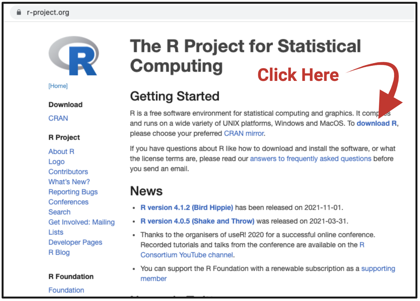
First, users should download R by navigating to the following website: https://www.r-project.org/
And then clicking the ‘download R’ link:
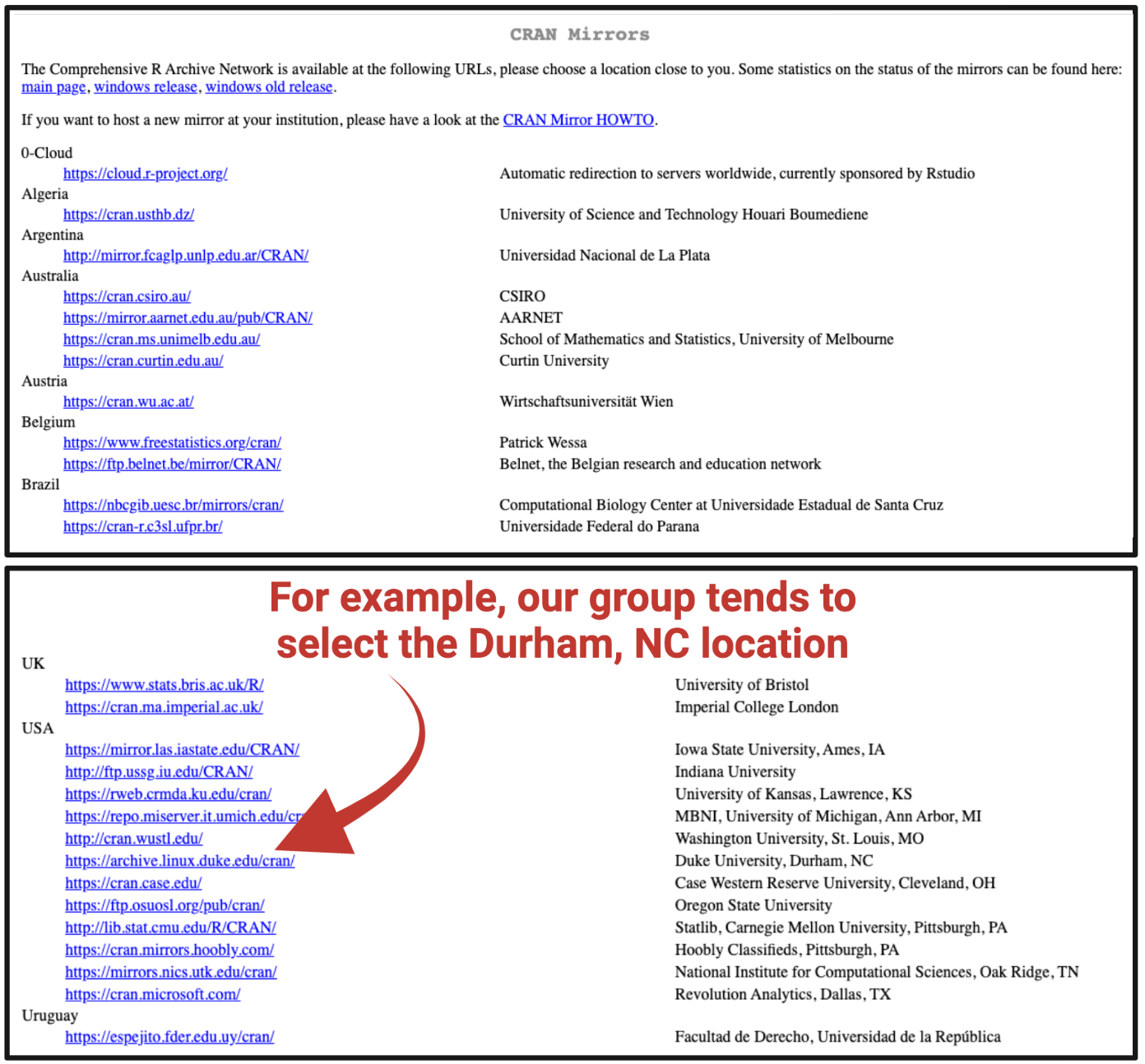
This link will navigate you to the CRAN mirror website. Click on the CRAN mirror location that seems closest to your usual location:
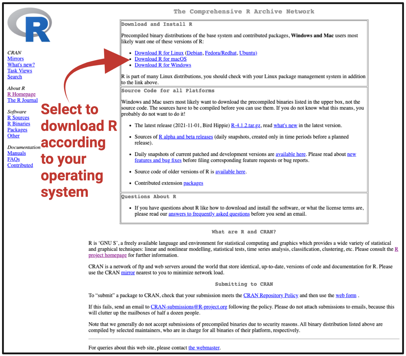
This will lead you to the selected CRAN Network website (here, https://archive.linux.duke.edu/cran/), where you will again select a download option:
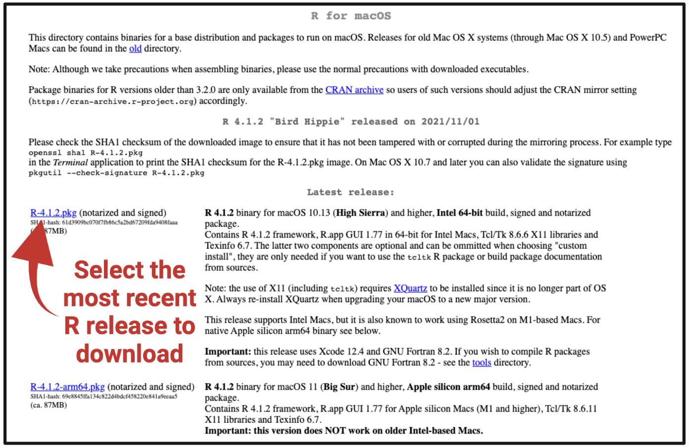
Then, select the top (representing the most recent) available .pkg file to download, and then install according to your computer’s typical program installation steps.
Downloading and Installing R Studio
What is R Studio? RStudio is an Integrated Development Environment (IDE) for R, which makes it more ‘user friendly’ when developing and using R script.
RStudio Desktop is a desktop application that can be downloaded for free, online. To download RStudio:
- Navigate to: https://rstudio.com/products/rstudio/download/
- Select the free RStudio Desktop option, and click “DOWNLOAD”
- Then download the top (most recent) RStudio Desktop option for your operating system
Here is a screenshot of what R script looks like within RStudio:
R Packages
One of the major benefits to coding in the R language is access to the continually expanding resource of thousands of user-developed packages that aid in improved data analyses and methods sharing. Packages have varying utilities, spanning basic organization and manipulation of data, visualizing data, and more advanced approaches to parse and analyze data, with examples included in all of the proceeding training modules.
In brief, packages represent compilations of code fitted for a specialized focus or purpose. These are often written by R users and submitted to the CRAN, or another host such as BioConductor or Github.
Examples of some common packages that we’ll be using throughout these training modules include the following:
- tidyverse: A collection of open source R packages that share an underlying design philosophy, grammar, and data structures of tidy data. For more information on the tidyverse package, see its associated CRAN webpage, primary webpage, and peer-reviewed article released in 2018.
- ggplot2: A system, within the tidyverse collection, for declaratively creating graphics. Users provide data they would like to plot, and then control how ggplot2 should map variables to aesthetics and define which graphical primitives to use; ggplot2 then drafts the corresponding visualizations. For more information on the ggplot2 package, see its associated CRAN webpage and R Documentation.
More information on these packages, as well as many others, is included throughout the training modules.
Downloading/Installing R Packages
R packages often do not need to be downloaded from a website. Instead, you can just load packages through running script in R, like:
install.packages(“tidyverse”)
library(tidyverse)
It is worth noting that a function can be queried in RStudio by typing a question mark before the name of the function. For example:
?install.packagesThis will bring up documentation in the viewer window.
Scripting Basics
Starting Code
RStudio will autofill function names, variable names, etc. by pressing tab while typing. If multiple matches are found, RStudio will provide you with a drop down list to select from, which may be useful when searching through newly installed packages or trying to quickly type variable names in an R script.
One of the first lines of code in any script will likely include the loading of packages needed to run the script. Here is an example line of code to load a package:
# Loading ggplot2 package (should already be installed as a base package)
library(ggplot2)
Many packages also exist as part of the baseline configuration of an R working environment, and do not require manual loading each time you launch R. These include the following packages:
- datasets
- graphics
- methods
- stats
- utils
Setting Your Working Directory
Another step that is commonly done at the very beginning of your code is setting your working direction. This points to where you have files that you want to upload / where the default is to deposit output files produced during your scripted activities.
You must set the working directory to a local directory where data are located or output files will be saved.
To view where your current working directory is (by default), run the following:
Show your working directory
getwd()To set the location of your working directory, run the following:
Set your working directory
setwd("/filepath to where your input files are")Note that in macOS, filepaths use “/” as folder separaters; whereas in PCs, filepaths use “\”.
Importing Files
After setting the working directory, importing and exporting files can be done using various functions based on the type of file being read or written. Often, it is easiest to import data into R that are in a comma separated values / comma delimited file (.csv) or tab / text delimited file (.txt).
Other data types such as SAS data files, large .csv files, etc. may require different functions to be more efficiently read in and some of these file formats will be discussed in future modules.
# Read in the .csv data that's located in our working directory
csv.dataset <- read.csv("Module1_1/Module1_1_ExampleData.csv")

# Read in the .txt data
txt.dataset <- read.table("Module1_1/Module1_1_ExampleData.txt")
These datasets now appear as saved dataframes (“csv.dataset” and “txt.dataset”) in our working environment in R.
Viewing Data
After data have been loaded into R, or created within R, you will likely want to view what these datasets look like. Datasets can be viewed in their entirety, or datasets can be subsetted to quickly look at part of the data.
Here’s some example script to view just the beginnings of a dataframe, using the “head” function in R (a part of the baseline packages)
head(csv.dataset)## Sample Var1 Var2 Var3
## 1 sample1 1 2 1
## 2 sample2 2 4 4
## 3 sample3 3 6 9
## 4 sample4 4 8 16
## 5 sample5 5 10 25Here, you can see that this automatically brings up a view of the first five rows of the dataframe.
Another way to view the first five rows of a dataframe is to run the following:
csv.dataset[1:5,]## Sample Var1 Var2 Var3
## 1 sample1 1 2 1
## 2 sample2 2 4 4
## 3 sample3 3 6 9
## 4 sample4 4 8 16
## 5 sample5 5 10 25Expanding on this, to view the first 5 rows x 2 columns, run the following:
csv.dataset[1:5,1:2]## Sample Var1
## 1 sample1 1
## 2 sample2 2
## 3 sample3 3
## 4 sample4 4
## 5 sample5 5To view the entire dataset in RStudio, use the “View” function:
View(csv.dataset)Exporting Data
Now that we have these datasets saved as dataframes, we can use these as examples to export data files from the R environment back into our local directory.
There are many ways to export data in R. Data can be written out into a .csv file, tab delimited .txt file, RData file, etc. There are also many functions within packages that write out specific datasets generated by that package. To write out to a .csv file:
write.csv(csv.dataset, "Module1_1_SameCSVFileNowOut.csv")To write out a .txt tab delimited file:
write.table(txt.dataset, "Module1_1_SameTXTFileNowOut.txt")R also allows objects to be saved in RData files. These files can be read into R, as well, and will load the object into the current workspace. Entire workspaces are also able to be saved.
# Read in saved single R data object (note that this file is not provided, just example code is for future reference)
r.obj = readRDS("data.rds")

# Write single R object to file (note that this file is not provided, just example code is for future reference)
saveRDS(object, "single_object.rds")

# Read in multiple saved R objects (note that this file is not provided, just example code is for future reference)
load("multiple_data.RData")

# Save multiple R objects (note that this file is not provided, just example code is for future reference)
save(object1, object2, "multiple_objects.RData")

# Save entire workspace
save.image("entire_workspace.RData")

# Load entire workspace
load("entire_workspace.RData")
Concluding Remarks
Together, this training module provides introductory level information on installing and loading packages in R. Scripting basics are also included, such as setting a working directory, importing and exporting files, and viewing data within the R console / RStudio environment. Additional resources that provide introductory-level information on coding in R include the following:
- Coursera provides a lot of materials on learning how to program in R: https://www.coursera.org/learn/r-programming & https://www.coursera.org/courses?query=r
- Stack overflow is a discussion forum for an online community of coders to discuss coding problems/challenges and ways to overcome these problems/challenges: https://stackoverflow.com/questions/1744861/how-to-learn-r-as-a-programming-language
- Wonderful tutorials are available online, like this one on ‘R for Data Science’: https://r4ds.had.co.nz/
- BioConductor provides package-specific help: https://www.bioconductor.org/
- An abundance of other resources are available online just by googling!
Comments
R allows for scripts to contain non-code elements, called comments, that will not be run or interpreted. Comments are commonly included when annotating code, or describing what your code does, where your data came from, and just general textual reminders throughout the script.
To make a comment, simply use a # followed by the comment. A # only comments out a single line of code. In other words, only that line will be commented and therefore not be run, but lines directly above/below it still will be
Comments are useful to help make code more interpretable for others or to add reminders of what and why parts of code may have been written.